Biomedical Engineering Reference
In-Depth Information
-
3
3
10
3
2.5
K
1
2
J
H
F
D
C
I
G
E
0.8
0.6
0.4
0.2
0
1.5
1
0.5
0
B
80
60
0
100
A
40
20
80
20
40
60
80
60
70
50
40
40
60
20
30
10
80
20
100
0
(a)
(b)
1
0.8
0.6
0.4
0.2
0
1.4
1.2
1
0.8
0.6
0.4
0.2
0
0
100
0
100
20
80
80
20
40
60
60
40
60
40
40
60
80
20
20
80
100
0
0
100
(c)
(d)
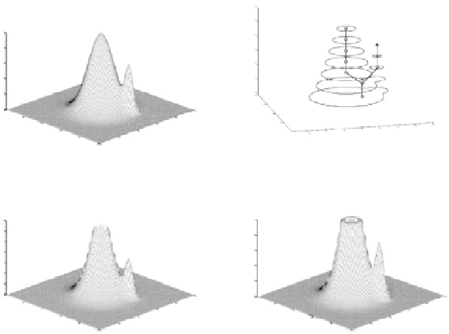
Figure 10.
Creation of the topological enhanced likelihood map: (a) original likelihood
map; (b) Max-Tree representation; (c) enhanced likelihood map without constraining max-
imum values; (d) final enhanced likelihood map.
The idea underlying the above formalization is to create a tree recursively
by analysis of the relationships among connected components of the thresholded
versions of the image. Figure 10 illustrates the process for
max-tree
creation. The
following explanation of the creation of the max-tree uses the notation for the flat
zones depicted in Figure 10b. In the first step, a threshold is fixed to the gray value
0, and all the pixels at level
h
=0are assigned to the root node
C
0
=
{
}
. The
pixels with values strictly superior to
h
=0form the temporal nodes (in our case,
TC
1
=
{
A
). Each temporal node is processed as if
it was the original image, and the new node will be the connected components
associated with the next level of thresholding
h
=1,
C
1
=
{
B, C, D, E, F, G, H, I, J, K
}
. Let's illustrate
a split. Suppose the process goes on until processing node
C
2
=
{
B
}
. The
temporal nodes at that point are the connected components strictly superior to
h
=2,
TC
3
=
{
C
}
and
TC
3
=
{
E, G, I
}
D, F, H, J, K
}
, and the associated nodes
at
h
=3are
C
3
=
{
and
C
3
=
{
.
Taking advantage of that concept, we now use the
Max-Tree representation
to
describe the function maps (characteristic function estimations). This representa-
tion allows further processing to be done keeping topological issues unchanged.
E
}
D
}