Biomedical Engineering Reference
In-Depth Information
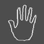
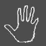
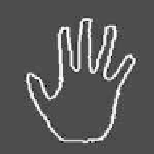
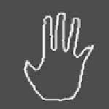
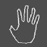
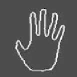
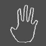
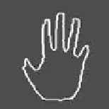
Figure 23.
The first row is the shape after using the weight factor only from the first
eigenshape. From left to right, the values of
w
are
−
0
.
3
and
0
.
3
. The second row is
the shape after using the weight factor only from the second eigenshape, and the same for
other rows. The only image in the second column is the average shape without any shape
variations.
with the shape's variability directly linked to the variability of the level set function.
Therefore, by varying
w
, Φ will be changed, which indirectly varies the shape.
However, the shape variability allowed in this representation is restricted to the
variability given by the eigenshapes. Several examples are illustrated in Figure
23 using different
w
to control the shape. From this example, the reader will find
it is very powerful to use different
w
for different eigenshapes to control shape
variations.
5.2. Model for Segmentation
As of now, the training procedure is concluded, and we can make full use of
the information after shape analysis. However, the implicit representation of shape
cannot accommodate shape variabilities due to a differences in pose. To have the
flexibility of handling pose variations,
p
is added as another parameter to the level
set function:
n
Φ[
w, p
](
x, y
)=Φ(
x, y
)+
w
i
Φ
i
(
x, y
)
,
(34)
i
=1