Biomedical Engineering Reference
In-Depth Information
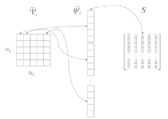
Figure 20.
Creating the shape-variability matrix
S
.
For segmentation, it is not necessary to use all the shape variabilities after
the above procedure. Let
k
n
, which is selected prior to segmentation, be the
number of modes to consider. In general,
k
should be chosen large enough to
be able to capture the main shape variations present in the training set. One way
to choose the value of
k
is by examining the eigenvalues of the corresponding
eigenvectors. In some sense, the size of each eigenvalue indicates the amount of
influence or importance its corresponding eigenvector has in determining the shape.
By looking at a histogram of the eigenvalues, one can estimate the threshold for
determining the value of
k
. However, an automated algorithm is hard to implement
as the threshold value for
k
varies for each different application. It is hard to
define a universal
k
that can be set. The histogram of the eigenvalues for the above
examples are listed in the Figure 21.
The eigenshapes are listed in Figure 22. In total there are 15 eigenshapes,
corresponding to the 15 eigenvalues. Only the 12 2D eigenshapes of the first 12
eigenvalues are listed in the figure.
A new level set function,
≤
k
Φ[
w
]=
¯
Φ+
w
i
Φ
i
,
(33)
i
=1
where
w
=
{
w
1
,w
2
,...,w
k
}
are the weights for the
k
eigenshapes with the
σ
1
,σ
2
,...,σ
k
}
variances of these weights
given by the eigenvalues calculated
earlier. Now we can use this newly constructed level set function Φ as the implicit
representation of shape. Specifically, the zero level set of Φ describes the shape,
{