Biomedical Engineering Reference
In-Depth Information
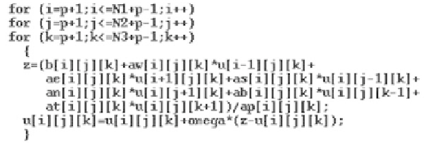
Figure 11.
One iteration of the standard serial SOR method.
built and stored in the same array
u
[
i
][
j
][
k
] by the procedure InitialSegmentation-
Function.
In every time step, the values of the discrete segmentation function are updated
in the DF nodes, solving iteratively the linear system with coefficients given by
(25). Figure 11 shows one iteration of the serial SOR method described in (25).
We can see the dependence of the currently updated value
u
[
i
][
j
][
k
] on its six
neighbours (the west, east, south, north, bottom, and top DF nodes). In every
iteration three of them should already be known (cf. (27)), so in parallel run every
consecutive process should wait until its preceding process is finished in order to
get the west values updated. Such dependence is not well suited for parallelization.
But there exists an elegant way to change the standard SORmethod to be efficiently
parallelized (see, e.g., [67]). It is possible to split all voxels to RED elements, given
by the condition that the sum of its indices is an even number, and to BLACK
elements, given by the condition that sum of its indices is an odd number. Then
the six neighbours of RED elements are BLACK elements (cf. Figure 12), and the
value of RED elements depends only on those of the BLACK elements, and vice
versa. Due to this fact, we can split one SOR iteration into two steps. First we
update RED elements and then BLACK elements, and this splitting is perfectly
parallelizable. Figure 13 shows one iteration of the so-called RED-BLACK SOR
method operating on RED elements.
After computing one RED-BLACK SOR iteration for the RED elements on
every parallel process, we have to exchange RED updated values in overlapping
regions, and then we can compute one iteration for BLACK elements. The data
exchange is implemented as shown in Figure 14 using non-blocking MPI Isend
and MPI Irecv subroutines. This iterative process is stopped using the condition
for a relative residual stated at the end of Section 3.4. Computing the initial residual
R
(0)
as well as all further residuals
R
(
l
)
, we have to collect partial information
from all the processes and send the collected value to all processes to check the
stopping criterion by every process. Figure 15 shows how the MPI Allreduce
subroutine is used toward that end in computing
R
(0)
. In fact, we compute by the