Biomedical Engineering Reference
In-Depth Information
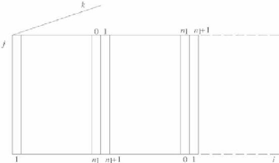
Figure 9.
Data distribution and its overlap over parallel processes.
three-dimensional array indexed by
i, j, k
. The 3D image is given in index ranges
i
=1
,...,N
1
+1,
j
=1
,...,N
2
+1,
k
=1
,...,N
1
+3. Let us suppose that
our computational domain, i.e., the domain where we update the segmentation
function, is equal to the image domain. Then the boundary positions with
i
=1,
i
=
N
1
+1,
j
=1,
j
=
N
2
+1,
k
=1,
k
=
N
3
+1are reserved for Dirichlet
boundary conditions and all the inner voxel positions correspond to DF nodes of
the 3D co-volume algorithm. In order to distribute the data (3D image as well as the
segmentation function), we define
n
1
=
n
procs
+1,
n
las
1
=
N
1
−
(
n
procs
−
1)
n
1
,
and we set
n
2
=
N
2
,
n
3
=
N
3
. Then on the root process with rank 0 we store
the first part of the 3D image as well as the first part of the discrete segmentation
function, namely, the array with indices
i
=1
,...,n
1
+1,
j
=1
,...,n
2
+1,
k
=1
,...,n
3
+1 (cf. Figure 9). The next process with rank 1 handles the next part
of the image and the segmentation function, namely, all 2Dslices
j
=1
,...,n
2
+1,
k
=1
,...,n
3
+1 locally indexed by
i
in the range
i
=0
,...,n
1
+1, where the 2D
slice with index
i
=0corresponds to the slice with index
i
=
n
1
in the root process
(cf. Figure 9). This is similar for further processes, with the only difference that on
the last process with rank
n
procs
−
1 the index
i
of the last 2D slice is
n
last
N
1
instead
1
of
n
1
. The merging of all 2D slices for
i
=1
,...,n
1
(
n
last
on the last process)
from all the subsequent processes gives the non-distributed complete 3D image as
well as the complete segmentation function. In order to solve iteratively the linear
system and to compute its coefficients, we need the overlap. The overlap in which
it is necessary to exchange information between neighbouring processes is given
by the slices
n
1
,n
1
+1and slices 0
,
1 of subsequent processes (cf. Figure 9).
As a first example showing how the data distribution is realized, we present the
procedure for the parallel reading of the 3D image in Figure 10. In all subsequent
figures the value of parameter
p
=1. Depending on the rank of the process, we
1