Theoretical Background - Response of Flood Events to Land Use and Climate Change - page 16

Table 2.1 Different interpolations characteristics (modified information based on [ 18 , 19 ])

Method Principle Advantages Disadvantages Best suited scenario Schematic

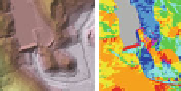
Nearest neighbor (NN) and thiessen polygon Selection of values at

closest data point

Ease of use Inaccurate in less densely

sampled scenarios

Densely sampled
environmental data

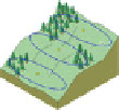
Triangulated irregular network (TIN) Set of conterminous with a

mass factor is used to
define the space

Ability to describe the surface at
different levels of resolution

In most cases, required visual
inspection and manual
control of the network

Dense and moderate
distribution of data
points

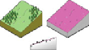
Polynomial regression (PR) Fits the variable of interest

to the linear
combination of
regressor variable

Simple model Model has poor ability to

predict outside the range
of data points

Moderately dense
sampling with
regard to global
variation

Global polynominal interpolation (GPI) Works by capturing coarse-

scale patterns in the
data, and fitting a
polynomial

Computationally less intensive Estimation errors increase

exponentially with
increasing complexity

Regions having sparse
data points and
simple data
patterns

Local polynominal interpolation Similar to GPI, but the

curve is fitted to a local
subset defined by
windows

Can interpolates short range variations Misses the global trends in data Well-distributed data

with no
discontinues

Trend surface analysis (TSA) Separates the data into

regional trends and
local variations

Assists in removal of broader trends
prior to further analysis

Edge effects and multi-co
linearity caused by spatial
autocorrelation

Important local trends
and not so
important global
trends