Results - Response of Flood Events to Land Use and Climate Change - page 152

0.02 0.03 0.04

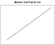
0.05 0.06 0.07

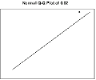
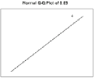
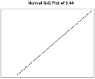
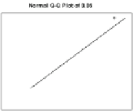
Fig. 6.20 Q-Q plot of regression standardized residual for different Manning's coefficient values

Table 6.11 Statistical analysis for different Manning's coefficient values

0.02 0.03 0.04 0.05 0.06 0.07

R .844 .735 .730 .845 .729 .732

R-square .712 .540 .533 .715 .531 .535

Standard error .203 .186 .215 .115 .256 .238

Table 6.12 PF and OF function for different Manning's coefficient values

0.02 0.03 0.04 0.05 0.06 0.07

Station 1 1 1 1 1 1

Time (hour) 24 24 24 24 24 24

Observed height water (m) 1.7 1.7 1.7 1.7 1.7 1.7

Simulated discharge (m 3 /s) 17.38 28.15 41.6 94.39 70.18 55.95

Simulated height water (m) 1.13 1.36 1.58 1.77 1.93 2.16

Penalty function 7.2 4.1 2.4 0.5 1.0 1.6

Object function 31.8 28.4 26.6 24.4 24.8 25.1

show that the error and level of uncertainty was at the lowest level. The results of
penalty function are shown in Table 6.12 .
Based on the results, the best agreement between observed and modeled height
of water was gained when the friction value of 0.05 was used for channel. The
optimization method was selected based on low object function.
In calibration procedure, all different friction values were applied in HEC-RAS
model simulation, and depth of water for different values was compared. The
successful modeling as expected before was the modeling with the friction value of
0.05 for river channel.