Environmental Engineering Reference
In-Depth Information
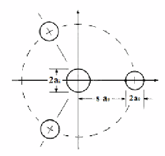
Fig. 3.10
Cross section of a
four-wire TDR probe [12]
realize and easy to insert; nevertheless, the analysis of the TDR waveform is some-
what more complicated and the region of influence is relatively high [34].
Fig. 3.11 shows the geometry and corresponding electrical fields of some typical
probe configurations. A three-rod probe and a two-rod probe are shown in Fig. 3.12
[13].
It must be pointed out that, when a noninvasive approach must be preserved, it is
possible to use surface probes, like the one shown in Fig. 3.13 [40]. Alternatively, it
is also possible to use antennas as sensing elements: this possibility will be discussed
in Sect. 5.6 [18].
It is worth mentioning that the probe configuration introduces some limitations
on the useful frequency range of analysis, mostly because of the geometric char-
acteristics. In particular, the TEM mode propagation assumption is true when the
operating wavelength is higher than the dimensions of the probe [26]. For example,
for a coaxial probe, the circumferential resonance frequency
f
up
,
circ
(below which
the TEM mode propagation assumption is valid) is given by
2
c
f
up
,
circ
=
)
π
√
ε
r
(3.18)
(
a
+
b
where
c
is the speed of light and
r
is the dielectric permittivity of the material filling
the probe
3
. Similarly, the longitudinal resonant frequency is given by [26]
ε
c
2
L
√
ε
f
up
,
long
=
(3.19)
r
where
L
is the length of the probe.
As a matter of fact, several probe configurations are commonly available on the
market; nevertheless, their configurations often do not allow an easy calibration
procedure to be performed. As will be detailed later in the topic, the calibration
procedure consists in measuring the reflected signal when some standard (known)
3
Equation (3.18) is equivalent to 2.10.


Search WWH ::

Custom Search