Basic Physical Principles - Broadband Reflectometry for Enhanced Diagnostics and Monitoring Applications - page 12

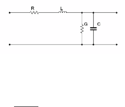
Fig. 2.1 Equivalent circuit
model for a transmission
line

define the secondary line constants , namely the propagation coefficient ( γ )andthe

characteristic impedance ( Z 0 ).
For an infinitely long line, the characteristic impedance Z 0 (which is defined as
the ratio of voltage V to current I in any position) can be written as

R

+ i ω L

Z 0 = (2.1)

G + i ω C

f is the angular frequency and i 2 where ω = 2 π = − 1.

The propagation coefficient is given by

γ = ( R + i ω L )( G + i ω C ) . (2.2)

It is useful to separate the imaginary part ( β ), which gives the phase-shift coefficient,

from the real part ( α ), which gives the attenuation coefficient:

R
2 Z 0 +

GZ 0
2

α = (2.3)

√ LC

β = ω

. (2.4)

For a lossless TL (i.e., when R = 0and G =

0), Z 0 can be written simply as

L

Z 0 =

/ C . (2.5)

From (2.5), it can be seen that for a lossless TL, the characteristic impedance is
purely resistive, although given by reactive elements ( C and L ). It is important to
point out that this does not mean that the line is a resistance.
In the following subsections, the most common types of TLs are considered,
namely coaxial, two-wire, and microstrip.

2.1.1 Coaxial Transmission Line

Coaxial lines are made of a central conductor with diameter a and a hollow outer
conductor with inner diameter b . The space between the conductors is usually filled
with a dielectric material: the electric and magnetic fields are confined within the