Environmental Engineering Reference
In-Depth Information
0.45
0.45
0.40
0.40
0.35
0.35
0.30
0.30
0.25
0.25
0.20
0.20
0
20
80
100
0
3
6
time (ns)
time (ns)
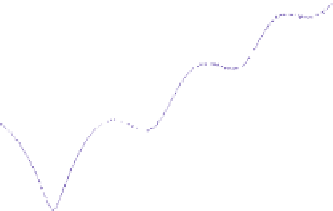
Fig. 6.10
TDR waveform of the biconical antenna for a 100 ns-long time window (left), zoom
of the initial portion of the waveform (right) [3]
0.6
0.5
0.4
0.3
0.2
|
S
11, ref
(
f
)|
T
w
= 30 ns
T
w
= 100 ns
0.1
0.0
0.0
0.5
1.0
1.5
2.0
2.5
3.0
f
(GHz)
Fig. 6.11
Comparison between
|
S
11
,
ref
(
f
)
|
and the
|
S
11
(
f
)
|
curves obtained from FD-
transformed data for different time windows (
T
w
), for the biconical antenna [3]
The analysis of the TDR waveform of the biconical antenna (reported in
Fig. 6.10) clearly shows that, differently from the previous case, the multiple re-
flections quickly die out and the signal reaches a steady-state condition in about
20 ns. Nevertheless, such a short
T
w
would not accurately represent the antenna re-
sponse at lower frequencies. In fact, Fig. 6.11 shows that even a 30 ns-long time
window, although providing overall accurate results, fails in accurately representing
the antenna response at low frequencies. On the other hand, if the time window is
too long, this will translate in inaccurate results at high frequencies. In fact, since the
maximum number of acquisition points is fixed, then the sampling period (
T
c
)may


Search WWH ::

Custom Search