Preliminaries - Control of Power Inverters in Renewable Energy and Smart Grid Integration - page 69

1 x 10 4

0.8

0.6

0.4

0.2

true poles
approximated poles

o

0

−0.2

−0.4

−0.6

−0.8

−1

−18 −16 −14 −12 −10 −8 −6 −4 −2 0

Re

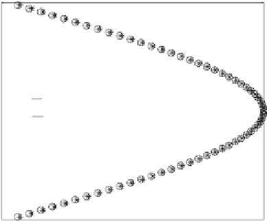
Figure 2.3 Poles of the internal model M for | k | ≤ 31. Note that the horizontal scale is much smaller
than the vertical scale, so that these poles are actually almost on the imaginary axis

The last approximation holds because if

τ d ω c

2 k π

1, then tan − 1

can be approximated by the

identity function.
The approximated poles and the true poles are shown in Fig. 2.3 for | k | ≤ 31. Actually,

j 2 τ the approximation is very good even for | k | ≤ 1000. Ideally, it is expected that s k = k .At

least, this is approximately true for small | k | .

2.2.3 Selection of the Delay in the Internal Model
In order to make Im s k ≈

2 π

τ

k , according to (2.8), τ d needs to satisfy

1
ω c τ.

2
d

τ = τ d τ −

(2.9)

Solving this equation,

1

4
ω c τ

1 ± −

τ d = τ. (2.10)

2

The solution with a minus sign is not reasonable, since it would lead to 1 and then many

of the approximations used earlier would break down. The reasonable solution corresponds to
the plus sign in (2.10), which leads to a good recommendation for

τ d ω c ≈

τ d as

2
ω c τ

1 + 1 −

1
ω c .

τ d ≈ τ = τ −

2