Environmental Engineering Reference
In-Depth Information
~
b
~
~
a
W
ξ
v
μ
w
e
+
P
u
d
~
W
d
C
u
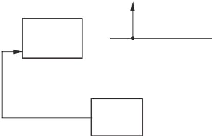
Formulation of the
H
∞
control problem
Figure 5.5
ξ
μ
ξ
μ
represented by
W
d
and weighting parameters
and
. The additional parameters
and
are
added to provide additional freedom in the design.
Assume that
W
is realised as
A
w
−
ω
c
B
w
ω
c
W
=
=
C
w
0
1
0
and
W
d
is realised (Wang 2008) as
A
d
B
d
C
d
D
d
−
2
T
s
4
T
s
W
d
=
=
,
1
−
1
where
T
s
is the sampling period. From Figure 5.5, the following equations can be deduced:
A B
1
B
2
C D
1
D
2
u
d
y
=
e
+
ξv
=
ξv
+
⎡
⎤
⎡
⎤
AB
2
C
d
0
B
1
B
2
D
d
v
u
⎣
⎦
⎣
⎦
.
=
0
A
d
00
B
d
(5.7)
CD
2
C
d
ξ
D
1
D
d
D
2
⎡
⎣
⎤
⎦
⎡
⎤
A
B
2
C
d
0
0
B
1
B
2
D
d
v
u
0
A
d
0
00
B
d
⎣
⎦
,
z
1
=
W y
=
(5.8)
B
w
C
1
B
w
D
2
C
d
A
w
B
w
ξ
B
w
D
1
B
w
D
2
D
d
D
w
C
1
D
w
D
2
C
d
C
w
D
w
ξ
D
w
D
1
D
w
D
2
D
d
z
2
=
μ
u
.
(5.9)


Search WWH ::

Custom Search