Voltage and Current H Repetitive Control - Control of Power Inverters in Renewable Energy and Smart Grid Integration - page 99

−L(j ω )

8

6

4

2

0

−2

−4

−6

−8

−2 −1 0 1 2 3 4 5 6

Re

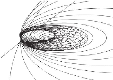
Figure 4.6 Nyquist plot of the loop gain − L ( j ω ) from u to u in Figure 4.2, shown for ω ≥ 0

where P yu is the plant transfer function from u to y given in (4.3) and M is the internal model
from (2.2). Hence,

A c B c 1
C c

A B 2
C 1 D 12

M A c B c 2

C c

A B 2
C 2 D 22

L = + .

0 0

The Nyquist plot of 0 is shown in Figure 4.6. This is a complicated curve

which does not encircle the critical point

− L ( j ω ) for ω ≥

1. The phase margin is about 40 ◦ and the gain −

margin is about 4 . 49 dB. Hence, the system has very good robustness w.r.t. to parameter

uncertainties.

4.5 Simulation Results
Simulations were done with MATLAB R /Simulink R . The solver used was ode23tb (stiff/TR-

s) and relative tolerance of 10 − 6 .
The phase of the grid voltage was assumed to be 0 ◦ . The voltage reference signal was
u ref

μ

BDF2) with variable steps (max. 1

t V, which is the same as the grid voltage. Thus, in the steady state and if
the grid was undistorted, there was no power exchanged between the microgrid and the grid.
A power controller was not included in the simulations. From the point of view of voltage
tracking, this does not matter because the power control loop is much slower. As mentioned
before, the voltage control of a three-phase inverter is decoupled into the voltage control of
three independent single-phase inverters when a neutral-leg controller is adopted to maintain
a balanced neutral line even if the loads on the microgrid are not balanced (Zhong et al.
2004a, 2006). Hence, there is no need to carry out simulations to demonstrate the three-phase
behaviour.

= 325 sin ω