Environmental Engineering Reference
In-Depth Information
1
2
40
40
20
20
0
0
−20
−20
−40
−40
90
90
45
45
0
0
−45
−45
−90
−90
10
0
10
2
10
4
10
6
10
8
10
10
10
12
10
0
10
2
10
4
10
6
10
8
10
10
10
12
Frequency (rad/sec)
Frequency (rad/sec)
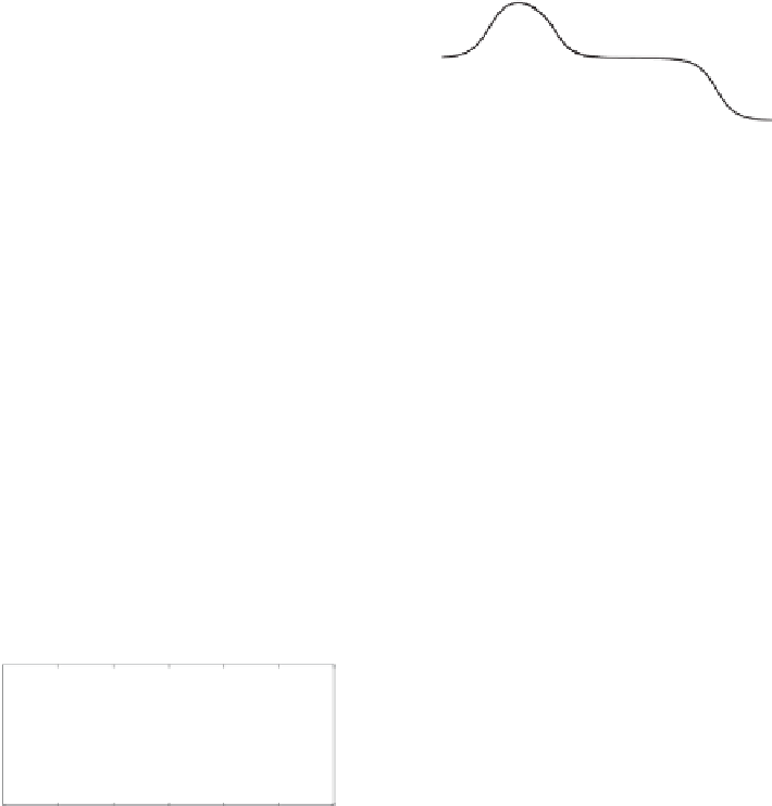
(a) Bode plots of
(b) Bode plots of
C
1
C
2
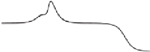
Figure 4.4
Bode plots of a nearly optimal controller
C
It is easy to check that
1 is satisfied for this
C
. Th
e pole
p
w
ith the highest
frequency creates a peak on the controller Bode plots at
T
ba
∞
<
| =
√
3
10
4
rad/s, as can be seen in Figure 4.5. This is well below half of the switching frequency
10
|
p
.
07
×
10
8
≈
1
.
752
×
10
4
rad/sec, which is the same as the sampling frequency to be used
to implement the controller, and hence the controller is implementable. This
C
is used as the
stabilising compensator in Figure 4.2 for the simulations presented in the next section.
The loop gain of the control system shown in Figure 4.2 is the transfer function
L
from
u
back to
u
. It is clear that
10
3
×
×
2
π
≈
6
.
28
×
C
M
0
01
P
yu
,
L
=
40
1
40
2
20
20
0
0
−20
−20
−40
−40
−60
−60
−80
−80
−100
−100
−120
−120
90
90
45
45
0
0
−45
−45
−90
−90
−135
−135
10
0
10
2
10
4
10
6
10
8
10
10
10
12
10
0
10
2
10
4
10
6
10
8
10
10
10
12
Frequency (rad/sec)
Frequency (rad/sec)
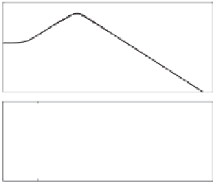
(a) Bode plots of
(b) Bode plots of
C
1
C
2
Figure 4.5
Bode plots of a more realistic suboptimal controller
C
from (4.7)


Search WWH ::

Custom Search