Environmental Engineering Reference
In-Depth Information
10
0
−10
−20
90
original
reduced
45
0
−45
−90
10
2
10
4
10
6
10
8
10
10
Frequency (rad/sec)
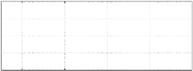
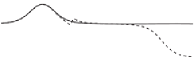
Figure 3.5
Bode plots of the original and reduced controllers
2265 for the
original controller. Hence, the closed-loop system is stable. The corresponding norm of the
transfer function from
The resulting
T
ba
∞
is 0
.
4634 for the reduced controller and
T
ba
∞
=
0
.
T
e
w
∞
=
T
e
w
∞
=
w
to
e
is
1
.
4434 and
1
.
0014, respectively. Using
the MATLAB
R
c2d (ZOH) algorithm, the discretised controller can be obtained as
1
.
7736(
z
−
0
.
953)
C
(
z
)
=
.
−
.
z
0
6005
3.4 Experimental Results
Various experiments were carried out in the grid-connected mode under different scenarios.
3.4.1 Synchronisation Process
As explained before, the grid voltages (
u
ga
,
u
gb
and
u
gc
) are feed-forwarded through a phase-
lead low-pass filter and added to the control signal for the inverter to synchronise with the grid.
The grid voltage
u
ga
, the inverter output voltage
u
A
and the voltage
e
u
dropped on the circuit
breaker and the grid interface inductor are shown in Figure 3.6 before and after the circuit
breaker was turned on. The inverter was started at
t
=
0 second and, immediately, it was
synchronised and connected to the grid.
3.4.2 Steady-state Performance
3.4.2.1 Without a Load
In the steady state, the current reference
I
d
was set at 3 A. The reactive power was set at 0
Va r (
I
q
=
0) so that the power factor is unity. Since there was no local load, all the generated


Search WWH ::

Custom Search