Biomedical Engineering Reference
In-Depth Information
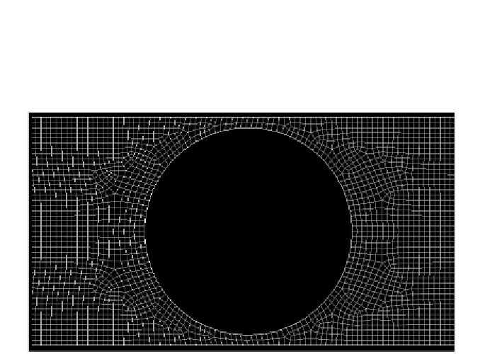
with a fixed mesh; only the mesh for the ball and zone immediately around it
moved. At the boundary between the dynamic and fixed portions of the mesh,
grid points were either generated or absorbed as necessary. Figure 29 shows
the mesh immediately surrounding the ball. A ball diameter of 40mm and an
inner tube diameter of 44mm was modelled.
Reproduced with permission. Copyright retained by Inderscience Publishers.
Figure 29. Mesh Immediately Surrounding the Ball.
Since the geometry is axi-symmetric, it is possible to compute the solution
with many fewer grid points than would be required for a complete 3D model.
The axi-symmetric model has approximately 2000 grid points. A very small
time step was used, Δt=0.0001 seconds, to capture the details of the highly
transient behaviour of the flow around the ball. 100 iterations per time step
were used and monitored computational residuals to ensure that the calculation
converged at each time step.
Figure 30 shows the calculated velocity contours around the ball at
t=0.001, t=0.002, t=0.003 and t=0.009 sec, respectively. The scale on the left
side of the Figure is the velocity in m/sec. The top three images show the
pressure pulse from the burst diaphragm reaching the ball. The images also
show the developing boundary layer. The fourth image shows a low velocity
area immediately in front of the ball and high-speed flow in the annular region
between the ball and the tube walls. This is analogous to the normal shock at
the throat of a conventional axi-symmetric convergent-divergent nozzle. The
flow is this area is well in excess of the speed of sound, which is
approximately 334 m/sec at sea level.