Concave Oligopolies - Nonlinear Oligopolies: Stability and Bifurcations - page 78

x

1

1

D (1)

x

x 2

D (1)

x 2

D (7)

D (7)

D (6)

D (6)

x 1 x 1

0 2

2 0

(a) N D 7 (b) N D 8

1

1

D (3)

D (2)

x 2

x 2

D (4)

D (3) 1

c

x

D (2)

1
c

D (1)

2

D (4)

c

x

D (7)

D (1)

D (7)

2

c

D (6)

D (6)

x 1 x 1

0 2 0 2

(c) N D 10 (d) N D 13

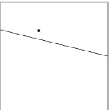
Fig. 2.14 Example 2.4; linear inverse demand and cost functions, the case of semi-symmetric
capacity constrained firms. A more detailed study of the bifurcations with respect to N. Note the
changing structure of the different regions of the map as N increases, and the border collision that
occurs as N increases from 8 to 10

As N is further increased the periodic points may cross the boundaries that sepa-
rate different regions, giving rise to border collision bifurcations that may change the
stability of the cycle involved and create new attractors. For example, in Fig. 2.14d,
obtained with N D 13, we can see that the periodic point c 2 has crossed the bor-
der, moving from region

.4/ . However this border collision did not cause a
change of stability of the 2-cycle, because after the border crossing the two periodic
points are in regions

.1/ to

D D

.7/ , so the 2-cycle remains stable with its multipli-
ers given by 1 .C 2 / D .1 a 1 / 2 , 2 .C 2 / D .1 a 2 / 2

.4/

D and D

(the two Jacobian matrices

J .4/ D J .7/ are triangular matrices). Nevertheless, in the bifurcation diagram of

Fig. 2.13 the occurrence of this border crossing can be easily detected around the
value N ' 12:7.

Example 2.5. In this example we return to the case of a quadratic price function

A Q 2 p A;

if 0 Q

if Q> p A;

f.Q/ D

0