Concave Oligopolies - Nonlinear Oligopolies: Stability and Bifurcations - page 75

1

x 1

0.4

0.5

x 2

0.3

0.4 0.5 0.6

L 2

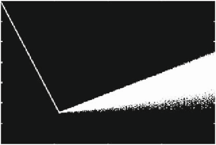
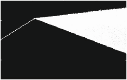
Fig. 2.11 Example 2.4; linear inverse demand and cost functions, the case of semi-symmetric
capacity constrained firms. Border collision bifurcations of x 1 (the output of firm 1)andx 2 (the
output of the other firms) as a function of L 2 (the capacity constraint of the other firms). Parameter
values are N D 21, A D 16, B D 1, a 1 D 0:2, a 2 D 0:3, c 1 D 6, c 2 D 6 and L 1 D 2

D

.1/ , where the equilibrium is unstable (since
N D 21 > N b .0:2;0:3/ D 12:6). The effect of this border collision is the sud-
den creation of a chaotic attractor that becomes larger and larger as the capacity
limit L 2 increases. Therefore, if firms in this industry invest in capacity, this can
cause quite dramatic effects in the asymptotic dynamics of the output sequences.
Whereas smaller capacity levels stabilized the industry, a small increase may lead
to complex dynamics. What about non-negativity of prices and profits in this situa-
tion? The profits of firm k are positive as long as x 1 C .N 1/x 2 <.A c k /=B,
and for the set of parameters used in Fig. 2.11 this means that all the profits are
positive as long as x 1 C 20x 2 <10. Non-negativity of prices is ensured because
Q max D L 1 C .N 1/L 2 max D 2 C 20 0:6 D 14 < 16 D A=B. Of course,
with these values of the parameters we could even consider capacities L 2 up to 0:7,
however this would lead to chaotic oscillations of greater amplitude. Consequently,
a larger proportion of the chaotic attractor in the regions of the strategy space would
be characterized by negative profits. For the one-dimensional model of Example 2.3

.7/ , where it is always stable, to

D