Concave Oligopolies - Nonlinear Oligopolies: Stability and Bifurcations - page 64

L

Rx ()

x

Tx ()

aL

x

Ac − 2 L Ac −

−

( NBN − ) − 1 ( NB −

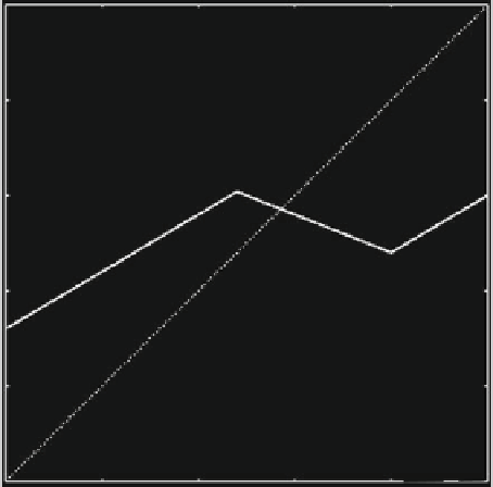
Fig. 2.3 Example 2.3; linear inverse demand and cost functions and identical capacity constrained
firms. The piece-wise linear map T.x/and reaction function R.x/

equilibrium is either at the boundary of the feasible set Œ0;L or in the interior, and
if the equilibrium is stable. The definition of R..N 1/x/ implies that 0 cannot be
equilibrium, so the equilibrium x is either interior or equals L.
As usual, the steady states of the adaptive adjustment process are the equilibria of
the underlying game, since T.x/ D x if and only if R..N 1/x/ D x.However,
the equilibrium might be located on the boundary. We account for this possibility by
writing the unique equilibrium point as

B.N C1/ ;L o . Its stability, under
the dynamic adjustment process governed by the iteration of the map T , depends on
the derivative of T , which has three segments with two different derivatives: 1 a
and 1

min n Ac

x D

a.N C 1/
2

. From the results of Appendix B we know that the equilibrium is

globally asymptotically stable of both j 1 a j and ˇ ˇ ˇ

ˇ ˇ ˇ

a.N C 1/
2

1 are less than one,

which is the case if 0<a< 4
N 1 .

We now turn to the asymptotic dynamics of the production sequences gener-
ated by T if, (1) the number of firms in the industry changes, and (2) each firm
is capacity-constrained. Figure 2.4 depicts a bifurcation diagram of output x with
respect to the number of firms N obtained with the parameters A D 16, B D 1,
a D 0:5, c D 6 and L D 1 (in all the numerical simulations in this subsection we
select the parameters such that NL A=B in order to ensure non-negative prices).
Observe that as long as .A c/=.B.N C 1// > L,thatisN<9, each firm produces

C