Chemistry Reference
In-Depth Information
1.3.5
Disconnected Basins
In all the examples encountered up to now, the basins of the corresponding attractor
were rather simple and were connected sets. As we shall now demonstrate, basins
can have a quite complicated structure. For example, they can be pierced by many
holes or may consist of areas without any connection. In such situations predicting
the long run outcome of the duopoly game where players use certain adjustment
processes to determine their production quantities over time is quite difficult. This
becomes particularly relevant when stochastic influences play a role.
In Fig. 1.16a we depict the situation after an increase in the adjustment speeds
from a
1
D
0:015, a
2
D
0:0165 (the values in Fig. 1.15b) to a
1
D
0:015; a
2
D
0:017.
After the contact of the curve LC
.b/
with the boundary of B.
1
/, a set indicated as
H
0
which belongs to the infeasible set B.
1
/ enters Z
2
(see the region indicated
by the arrow in Figs. 1.16a, b).
This means that points belonging to H
0
have two distinct preimages, say H
.1/
1
and H
.2/
1
, which are located on opposite sides of the curve LC
.b/
1
(the preimages of
inside B.
1
/ are located on LC
.b/
points exactly on the curve LC
.b/
1
). Obviously,
since H
0
belongs to the set B.
1
/, initial conditions belonging to H
.1/
1
and H
.2/
1
also lead to infeasible trajectories, since they are mapped into the infeasible set after
one iteration. The rank-1 preimages of H
0
constitute a so-called
hole
of B.
1
/
which is located entirely inside the feasible set (this hole is also called a “lake” in
Mira et al. (1996)). Since this hole, also referred to as the
main hole
, again lies inside
the region Z
2
, it also has two preimages. These smaller holes, denoted as H
.1/
and
2
6
6
x
x
2
Z
0
E
2
(1)
H
−2
()
b
LC
H
0
H
0
(1)
H
−
1
()
ω
11
−
(2)
H
−
1
E
(1)
2
H
−
Z
2
(2)
H
LC
(
b
)
−
2
LC
(
a
)
Z
4
4
x
1
x
E
1
2
0
6
0
1
(a)
(b)
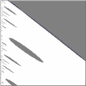
Fig. 1.16
The Cournot duopoly with a gradient type adjustment process and linear
demand/quadratic cost. Slightly higher speeds of adjustment than in the case of Fig. 1.15. The
critical curve LC
.b/
has crossed the basin boundary and a disconnected basin of attraction now
results. (
a
) The entire region. (
b
) A close up of the set H
0
and its preimages


Search WWH ::

Custom Search