Chemistry Reference
In-Depth Information
0.025
A
2
a
2
a
1
0
A
1
0.025
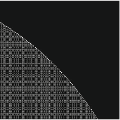
Fig. 1.13
The Cournot duopoly with a gradient type adjustment process and linear
demand/quadratic cost. The
hashed area
indicates the stability region of the interior Nash
equilibrium E in the .a
1
;a
2
/ plane of adjustment speeds
of .a
1
;a
2
/ inside the stability region, the Nash equilibrium E is an asymptotically
stable node. The boundary of this region represents a bifurcation curve at which
E loses asymptotic stability through a flip (or period doubling) bifurcation (see for
example Guckenheimer and Holmes (1983), or Lorenz (1995)). This bifurcation
curve intersects the axes in the points
;
.B
C
e
1
/x
1
;0
and A
2
D
0;
1
1
.B
C
e
2
/x
2
A
1
D
from which further information on the effects of the model's parameters on the local
asymptotic stability of E could be derived by further analysis.
So far we have only considered questions related to local asymptotic stability of
the interior equilibrium. But what can we say about the global dynamics? That is,
given that the interior Nash equilibrium is locally asymptotically stable, what can
be said about its basin of attraction, defined as the set of feasible initial conditions
which generate bounded and positive trajectories converging to E? In Fig. 1.14,
obtained with parameters A
D
450, B
D
30, c
1
D
c
2
D
275, e
1
D
e
2
D
11 and
speeds of adjustment a
1
D
0:01, a
2
D
0:012, the Nash equilibrium E
D
.2:57;2:57/
is locally asymptotically stable and its basin of attraction (or feasible set) is rep-
resented by the white area. The region in grey represents the basin of infinity,
denoted B.
1
/, that is the set of initial conditions that generates unbounded (and
negative), therefore “infeasible”, trajectories. The interior Nash equilibrium is not
globally asymptotically stable since not all initial conditions in the strategy space

Search WWH ::

Custom Search