Oligopolies with Misspecified and Uncertain Price Functions, and Learning - Nonlinear Oligopolies: Stability and Bifurcations - page 253

2.5 2.5

ε ε

2

2

( B , B )

ε 1

ε 2.5

0 2.5 0

1

(a) (b)

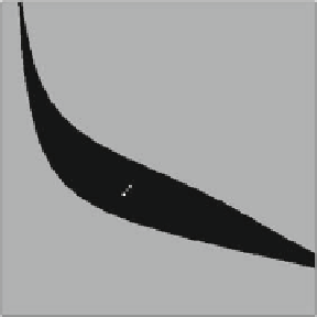
Fig. 5.7 The duopoly with heterogeneous players. From initial values in the white region the
system generates feasible trajectories, from initial values in the grey region , the trajectories become
infeasible. Here A 0:6.( a ) The equilibrium is a stable node with

one positive and one negative real eigenvalue. The speeds of adjustment are a 1 D

D 5, B D 1, c 1 D 0:5 and c 2 D

1.
( b ) The steady state becomes a saddle point and a stable cycle of period 2 emerges. The speeds of
adjustment are a 1 D

0:9 and a 2 D

0:9475 and a 2 D 1

is obtained with a higher value of the speed of adjustment a 1 , namely a 1 D 0:9475.
In this case, as expected on the basis of the local stability analysis, the steady state
is a saddle point, because a period doubling bifurcation has created a stable cycle of
period 2, represented by the two small dots in Fig. 5.7b. This means that none of the
two firms learns the demand and they keep on underestimating and overestimating
it. As a 1 =B and/or a 2 =B are further moved away from the stability region, the peri-
odic points move away from the unstable steady state, and so the amplitude of the
oscillations increases. Moreover, other local bifurcations may occur, at which also
the cycle of period two loses stability and more complex attractors may appear (for
example, the 2-cycle may flip bifurcate to give rise to a stable cycle of period 4,and
so on, until chaotic attractors appear after the well-known period-doubling cascade)
or the attractor may have a contact with the boundary of its basin of attraction and
disappear, after which the generic trajectory will be infeasible.
Let us now consider the case of a larger difference between the cost parameters
c 1 and c 2 , so that the condition (5.112) is satisfied and, consequently, the stabil-
ity region is also bounded by a portion of the curve H where a Neimark-Hopf
bifurcation occurs. By setting A D 5, B D 1, c 1 D 0:5 and c 2 D 1:3,asin
Fig. 5.6b, we consider a set of parameters inside the stability region, namely a 1 D 1,
a 2 D 0:9. Hence, the equilibrium, shown in Fig. 5.8a with its feasible set of attrac-
tion, is a stable focus (complex conjugate eigenvalues of modulus less than 1). As
expected, if we increase a 1 and/or a 2 ,sothat.a 1 =B;a 2 =B/ crosses the boundary
H of the stability region, a supercritical Neimark-Hopf bifurcation occurs, at which
the steady state is transformed into an unstable focus, and an attracting closed invari-
ant curve is created around it (see Fig. 5.8b, obtained with a 1 D 1:17 and a 2 D 0:9).