Chemistry Reference
In-Depth Information
costs c
1
=c
2
. Feasible, that is bounded and non-negative, trajectories of the best reply
dynamics are obtained provided that c
1
=c
2
2
Œ4=25;25=4
D
Œ0:16;6:25.
M
ore-
ove
r,
the Nash equilibrium (5.59) is stable if and only if c
1
=c
2
2
.3
2
p
2;3
C
2
p
2/
'
.0:17;5:83/.Ifc
1
=c
2
exits this interval then the Nash equilibrium loses
sta
bi
lity via a
p
eriod doubling bifurcation. If c
1
=c
2
falls outside the interval .3
2
p
2;3
C
2
p
2/ then the asymptotic dynamics may converge to periodic cycles or
even exhibit chaotic motion around the Nash equilibrium. Consequently, in terms
of the cost parameters convergence to the Nash equilibrium is obtained for a wider
range of parameters in the model with LMA than in the case where firms know the
true nonlinear demand and at each time step play the best reply. This insight could be
summarized in the statement that
less information implies more stability
.However,
it should be noticed that this result is obtained through a comparison of the stability
region in the space of unit cost parameters .c
1
;c
2
/ in the following sense: the Nash
equilibrium
x
is stable for each selection of the parameters .c
1
;c
2
/ f
or
the mo
de
l
with LMA, whereas stability only holds in the subset c
1
=c
2
2
.3
2
p
2;3
C
2
p
2/
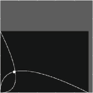
in the case of best reply adjustment. Quite different conclusions may be reached if
we compare the basins of attraction. In fact, with cost parameters such that the Nash
equilibrium is stable under both adjustment mechanisms, larger basins of attraction
can be observed for the model with best reply. This is illustrated in Fig. 5.4. The
white regions represent the basins of attraction of the corresponding stable Nash
equilibrium in the best reply model (case (a), where we also depict the best replies)
and the LMA model (case (b)). The grey regions represent the set of initial condi-
tions that generate infeasible trajectories. Obviously, the basin is larger in the former
case.
1.5
1.5
x
2
x
2
x
*
x
*
x
1
x
1
0
0
1.5
1.5
(a)
(b)
Fig.
5.4
Local
monopolistic
approximation
with isoelastic
demand
and
linear
cost.
Here
c
1
D
0:7.(
a
) Nash equilibrium in the best reply model. (
b
) The LMA case. In both
cases, the
white region
represents the basin of attraction of the stable equilibrium, initial values in
the
grey region
generate infeasible trajectories
1;c
2
D


Search WWH ::

Custom Search