Modified and Extended Oligopolies - Nonlinear Oligopolies: Stability and Bifurcations - page 167

Assume now that the price function f and cost functions C k satisfy the con-
ditions (A)-(C) of concave oligopolies given at the beginning of Sect. 2.1. Then
1<r k 0 for all k.Letg./ denote the left hand side of (4.45) and assume that
all a k >0 and the 1 a k .1 C r k / values are different, otherwise we can add the
terms with identical denominators similarly to (2.24). Clearly,

N

X

lim g./ D r k .a k C ˇ S / 0;

!˙1

k D 1

and it is positive unless all r k D 0, which case is excluded from discussion. Further-
more

lim

0 g./ D˙1 ! 1 a k .1 C r k / ˙

and

X

N

a k r k .1 .a k C ˇ S /.1 C r k //
.1 a k .1 C r k / / 2

g 0 ./ D <0

k D 1

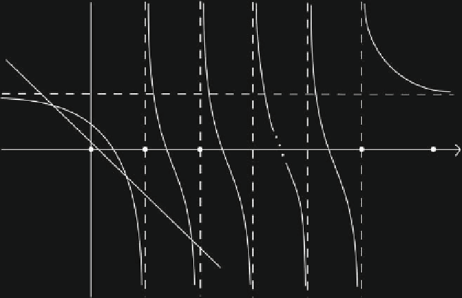
by assuming that for all k, .a k C ˇ S /.1 C r k /<1. The graph of g./ is shown
in Fig. 4.11, and notice that under this assumption all poles of g are positive and
below 1. Notice also that

1 − a 1 (1 + r 1 ) 1 − a 2 (1 + r 2 ) 1 − a S (1 + r S )

1

λ

0

β−λ

Fig. 4.11 The oligopoly model with intertemporal demand interaction and best reply dynamics
with adaptive expectations in the discrete time case. Graph of g./ the roots of which are the
eigenvalues of the Jacobian matrix