Chemistry Reference
In-Depth Information
0.6
x
1
0.1
0.6
x
2
0.1
0
a
2
1
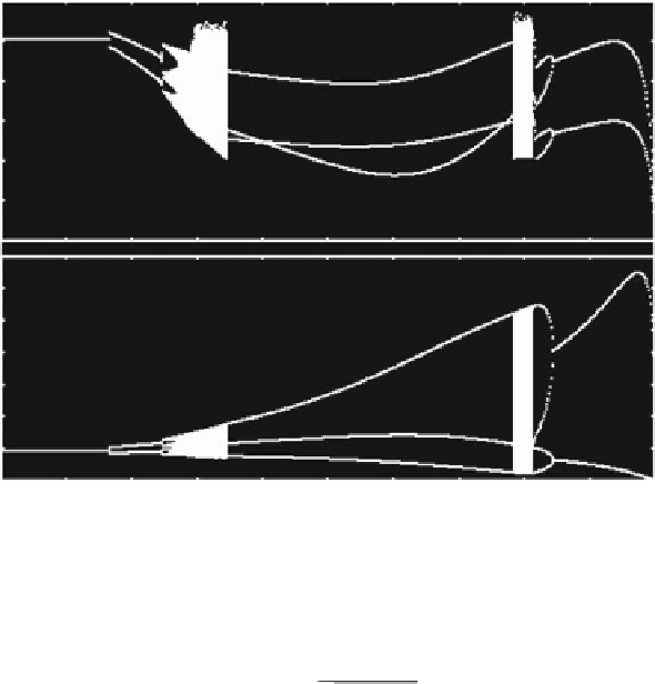
Fig. 3.7
Example 3.4; discrete time oligopoly with isoelastic demand and linear cost functions -
the semi-symmetric case. Bifurcation diagrams of outputs x
1
;x
2
with respect to a
2
with the number
of firms held fixed at N
D
23. The parameters are otherwise as in Fig. 3.6
1
a
1
a
1
2.N 1/
.N
1/
!
;
p
5.N 1/x
2
J
.2/
D
1
a
2
0
1
a
1
0
01
;
J
.3/
D
a
2
and
!
:
1
a
1
0
a
2
p
2
2/x
2
1
1
a
2
C
.N
2/a
2
p
2
2/x
2
1
J
.4/
D
p
3Œx
1
C
p
3Œx
1
C
.N
.N
D
.1/
and
D
.4/
may we have points at which the Jacobian
Notice that only in regions
determinant vanishes.
After the foregoing preparations, we are now in a position to describe some bor-
der collision bifurcations as well as some methods to bound chaotic attractors that
involve the lines of non-differentiability for a specific numerical example. Let us
start from the set of parameters used to obtain the bifurcation diagram Fig. 3.7, that
is N
D
23, A
D
16, a
1
D
0:4, c
1
D
5, c
2
D
6, L
1
D
L
2
D
2. From the second sta-
bility condition in (3.15) we can deduce that at a
2
D
21120
127781
'
0:165 the Nash
equilibrium x loses stability through a flip bifurcation, at which it becomes a saddle
point, and a stable cycle of period 2 is created around it. Just after this bifurcation,


Search WWH ::

Custom Search