Chemistry Reference
In-Depth Information
1
1
x
2
D
(2)
D
(1)
x
1
x
0.
1
D
(9)
x
2
0.5
0.7
0.5
1
100
150
x
1
Time
(a)
(b)
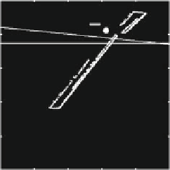
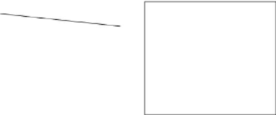
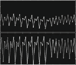
Fig. 2.19
Example 2.5; quadratic price and linear cost functions. The semi-symmetric case.
(
a
) The attractor associated with Fig. 2.18 for a
1
D
0:8.(
b
) The time series along the chaotic
attractor. Note the correlation between x
1
and x
2
in both figures
quantities of the other (symmetric) firms in the following sense: periods where
the output x
1
.t/ of firm 1 is high are associated with periods where x
2
.t/ is high.
The same can be observed for periods with low output values (see also Fig. 2.19b,
where the asymptotic values of typical time series for x
1
.t/ and x
2
.t/ moving along
the chaotic attractor are shown). In this case, the firms' actual production choices
and their expectations of the joint outputs of the other firms move jointly up and
down and enable the observer to make a qualitative prediction of what to expect
next, an increase in industry output or a decrease.
2.4
Gradient Adjustments
In this section we briefly examine the gradient adjustment processes introduced in
Sect. 1.2. Further examples and applications of gradient dynamics will be presented
in the following chapters. In the case of the classical Cournot model without cost
externalities the discrete time gradient adjustment process (1.32) becomes
x
k
.t/f
0
N
x
i
.t/
!
C
f
N
x
i
.t/
!
C
k
.x
k
.t//
!
;
X
X
x
k
.t
C
1/
D
x
k
.t/
C
˛
k
i
D
1
i
D
1
(2.39)
and the continuous time gradient adjustment process (1.33) simplifies to
x
k
.t/f
0
N
x
i
.t/
!
C
f
N
x
i
.t/
!
C
k
.x
k
.t//
!
: (2.40)
X
X
x
k
.t/
D
˛
k
i D1
i D1

Search WWH ::

Custom Search