Biomedical Engineering Reference
In-Depth Information
12.4.2 Numerical results
We present two test cases on simplified geometries, solved again with the library
LifeV
. These test cases have the role of assessing the overall performances of the
method on synthetic data, in view of a more extensive analysis using real medical im-
ages. The “synthetically measured” displacement field
η
fwd
is therefore generated
by a preliminary numerical simulations with a prescribed Young's modulus. Succes-
sively, the data are perturbed in order to mimic the presence of noise. The noise is
generated with a uniform distribution
U
,where
−
η
M
2
ξ
,
η
M
η
M
=
max
x
,
t
|
η
fwd
(
x
,
t
)
|
.
2
ξ
Smaller values of the parameter
represent a greater incidence of the noise.
In the first set of simulations (already reported in [83]), we solve the problem in a
cylinder of radius
R
ξ
6
cm
. The computation is performed in
2D under the assumption of axial symmetry of the problem. We impose the pressure
drop
=
0
.
5
cm
and height
H
=
10
4
dyne
cm
2
Δ
p
=
/
for the first 5
ms
between the inlet and the outlet of the
cm
2
cm
2
vessel. We set
ρ
f
=
1
g
/
,
ρ
w
=
1
.
1
g
/
,
μ
=
0
.
035
Poise
,
h
s
=
0
.
02
cm
,
E
=
10
6
dyne
cm
2
,
1
001
s
.
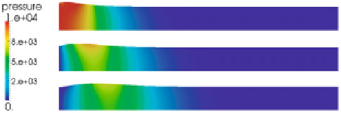
Fig. 12.11 shows the geometry and the pressure along a longitudinal section of
the cylinder, for different time instants.
The optimization problem has been solved by using the BFGS algorithm over
10 time steps, corresponding to the first 10
ms
of the simulation. We run the op-
timization problem for 10 realizations of the noise. In Table 12.2, we report the
average over the 10 realizations of the estimated values of
E
and the relative error.
Different initial guesses
E
0
and different
.
3
·
/
ν
=
0
.
3and
Δ
t
=
0
.
ξ
are considered. These results show that
for large values of
ξ
, the estimate obtained by the method is accurate. A reasonable
Fig. 12.11.
2D axisymmetric case, Forward simulation. Geometry at time
t
=
5
ms
,
t
=
7
ms
and
cm
2
t
=
9
ms
. Colored with blood pressure, in
dyne
/
Table 12.2.
Standard deviation of the ten estimates (to be multiplied by 10
6
, top) and mean per-
centage error (bottom) for different values of the initial guess
E
0
for the Young's modulus and of
the percentage
P
. Exact
E
is 1
.
3
·
10
6
dyne
/
cm
2
↓
E
0
\
ξ
→
10
5
3.3
2.5
10
7
dyne
cm
2
/
1
.
302
±
0
.
027
1
.
314
±
0
.
054
1
.
330
±
0
.
085
1
.
357
±
0
.
103
0
.
2%
1
.
1%
2
.
3%
4
.
4%
10
5
dyne
cm
2
/
1
.
303
±
0
.
027
1
.
315
±
0
.
056
1
.
330
±
0
.
087
1
.
348
±
0
.
115
0
.
2%
1
.
1%
2
.
3%
3
.
7%