Biomedical Engineering Reference
In-Depth Information
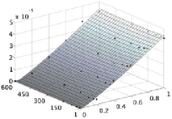
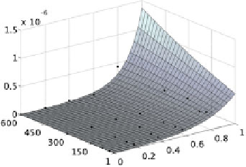
Fig. 11.3.
A visual comparison of
D
(
φ
,
x
)
,D
(
φ
,
x
)
with the entries of Tables 11.3 and 11.4
w
w
i
w
respectively. The control points are visualized with dots
As a result of that we obtain,
2
w
D
i
(
φ
w
,
x
)=
exp
(
−
4
.
531
+
5
.
483
φ
w
+
0
.
000642
x
−
0
.
00074
φ
w
x
−
0
.
693
φ
00000115
x
2
2
w
x
φ
w
x
2
w
x
2
2
−
0
.
+
0
.
002
φ
−
0
.
000004
+
0
.
000005
φ
)
that ensures that
D
i
(
φ
w
,
x
)
is always positive. A visual comparison of the interpolants
D
w
(
φ
w
,
with the corresponding control points, that are entries of Ta-
bles 11.3 and 11.4 respectively, is reported in Fig. 11.3.
The results of numerical simulations for
x
)
,D
i
(
φ
w
,
x
)
40
31
˜
ρ
w
(
t
,
z
)
,
ρ
(
t
,
z
)=
∑
i
ρ
i
(
t
,
z
)
,
ρ
=
40
i
=
31
10
1
10
i
=
1
∑
ρ
i
(
t
,
z
)
,
ρ
=
∑
ρ
i
(
t
,
z
)
are reported in Fig. 11.4. Depending on the value
of the Thiele modulus,
Λ
, different modes of degradation and erosion occurred. For
Λ
=
PLA
17000 diffusion occurs at a much faster rate than the chemical reaction
and water have saturated the polymer across the entire thickness before significant
scission takes place (Fig. 11.4 top-left). Polymeric byproducts are produced almost
homogeneously across the thickness of the coating and their consequent diffusion
is responsible for conferring bulk erosion characteristics to the behaviour of the
reaction-diffusion system (Fig. 11.4 bottom-left). Polymeric density ˜
decreases in
a homogeneous fashion across the coating as smaller chains diffuse away (Fig. 11.4
top and bottom-right). Such qualitative interpretation of polymer degradation can
be profitably complemented with the analysis of the evolution of the system in the
lumped state space
ρ
, reported in Fig. 11.5. It shows that, because of fast wa-
ter absorption and subsequent hydrolysis, the average degree of polymerization
x
quickly decreases and the water content of the mixture
(
φ
w
,
x
)
φ
w
progressively increases.
At the end of the process, most of the polymer in the mixture is in the range of small
sub-fractions as confirmed by Fig. 11.4 bottom-left.
Further information is obtained by analyzing how the mean value of the partial
density of water and polymer, respectively defined as follows,
L
0
ρ
w
(
L
1
L
1
L
˜
ρ
w
(
¯
t
)=
t
,
z
)
dz
,
ρ
=
ρ
(
˜
t
,
z
)
dz
.
0