Applications to Real Measured Data - Introduction to Imaging from Scattered Fields - page 129

(a)

2 λ

(b) (c)

[ k -space] [ k -space]

×10 4 ×10 4

9
8
7
6
5
4
3
2
1

2

-60 -60

1.8

-40 -40

1.6

1.4

-20 -20

1.2

1

0 0

0.8

20 20

0.6

0.4

40 40

0.2

60
-60

60
-60 -40 -20 0 2040 0 -40 -20 0 2040 0

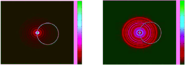
Figure 9.15 The k -space coverage for cylinder of radius 2 λ : (a) Target cylinder, (b) k -space coverage for weak
scattering cylinder, and (c) k -space coverage for strong scattering cylinder.

can view this as an effective sampling of k -space that results in increasingly
spread out high spatial frequency data locations as k increases, as indicated in
Figure 9.15, and one might justifiably expect that an increased sampling rate
would be necessary in order to capture this information.
Note that for the same geometrically sized cylindrical object in the images
above, the k -space coverage varies dramatically as a function of the permit-
tivity of the cylinder. For this reason, small radius Ewald circles will cover
mostly low spatial frequencies while large radius Ewald circles will capture
information about both low and many high spatial frequencies. The radius
of the Ewald sphere in k -space changes with varying incident frequencies.
Hence, the mapping between the scattered field data on these circles and the
k -space representation of the two different V Ψ shown here results in differ-
ent regions of k -space being sampled. Small incident k values only map on to
lower spatial frequencies. Each estimate obtained from a given incident fre-
quency can add information about different spatial frequencies and, in prin-
ciple, should help in improving reconstruction quality.
It is also noted that the wrong value for the background permittivity is
observed in Figure 9.11e. It has been postulated (Shahid, 2009) that the con-
trast reversal and incorrect surrounding permittivity level could be caused by
the limited sampling of the scattered field for these objects, becoming increas-
ingly limited as k increases for a given source-receiver set of locations. The
problem of limited data and undersampling can be addressed by using the
PDFT algorithm. Figure 9.16 shows the comparison of DFT and different prior
functions incorporated into the PDFT reconstructions. It is evident from
Figure 9.16b that the contrast of the reconstruction is incorrect when using