Born Approximation Observations - Introduction to Imaging from Scattered Fields - page 96

0

0.03

50

0.025

100 0.02

0.015

150

0.01

200

0.005

250

0 50 100 150 200 250

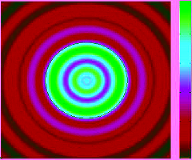
Figure 6.6 The resulting reconstructed image for a 2-D cylinder with a positive value of 1 for the permeability
and a varying negative values for the permittivity. All images look virtually the same regardless of the (negative)
value for the permittivity.

as p is now an imaginary number and, as is well known, this corresponds
to a very lossy or evanescent case of a wave. Thus, when the permittivity is
negative and the permeability is positive, the Q relationship breaks down and
one would expect no resonances to be predicted. If this condition is simulated
using the methods above, the reconstructed images for all of the values in the
range of permittivities look like the image in Figure 6.6, which is very poor. To
correctly model a negative index material, the permeability value needs to also
be set to −1 when the permittivity value is negative. This allows for the nega-
tive root to be selected for p which yields a real-valued representation for Q .
This gives results consistent with those of the simulation, as seen in Figure 6.5.

ReFeRenCeS
Jones, W. B. 1988. Introduction to Optical Fiber Communication Systems.
New York: Holt, Rinehart, & Winston, Inc.
Kasap, S. O. 2001. Optoelectronic Devices and Photonics: Principle and
Practices. New Jersey: Prentice-Hall.
Lustig, M., Donoho, D., and Pauly, J. M. 2010. Sparse MRI: The application
of compressed sensing for rapid MR imaging. Magnetic Resonance In
Medicine , 58 (6), 1182-1195.
Miller, D. A. 2007. Fundamental limit for optical components. Journal of
Optical Society of America B , 24 (10), A1-A18.
Ritter, R. S. 2012. Signal Processing Based Method for Modeling and Solving
Inverse Scattering Problems. University of North Carolina at Charlotte,
Electrical Engineering. Charlotte: UMI/ProQuest LLC.