Hardware Reference
In-Depth Information
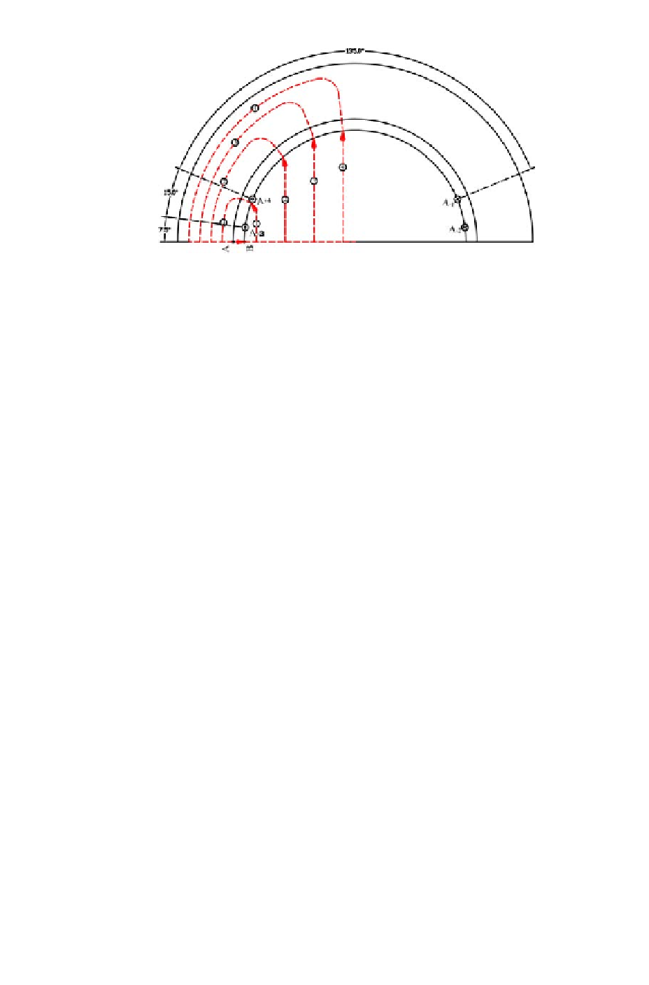
Figure 4.10: Cross-section of the motor showing the integration loops
It is easily observed from Figures 4.10 and 4.11 that, in the range (0
◦
, 7.5
◦
),
the right side of equation 4.30 is zero and therefore F
g
(θ)iszerointherange
(0
◦
, 7.5
◦
). At θ =7.5
◦
, F
g
(θ) jumps to the value W
c
I and remains the same
for the range (7.5
◦
, 22.5
◦
) because no other conductors are included in the
loop. Similarly, F
g
(θ) jumps to 2W
c
I at θ =22.5
◦
and remains the same for
◦
◦
the entire range of (22.5
). It can be easily comprehended that as θ
continues to change from 0
◦
to 360
◦
, the airgap MMF F
g
(θ)showssudden
“jumps” at all positions where the conductors are located. So the MMF as
a function of θ is shown by the waveform of Figure 4.12. For the electric
machines, the conductors are installed in the stator slots. Therefore, it is not
difficulttodrawtheMMFcurveintherange(0
◦
, 360
◦
), even for the motor with
complicated distribution windings. As all the armature winding are installed
in the stator slots, the MMF jumps can be assumed to occur at the position of
slot centers. It was shown in equation 4.19 that the MMF F
g
(θ) is proportional
to the airgap
fl
ux density B
g
(θ). Therefore, the waveform shown in Figure 4.12
also represents the variation of airgap
fl
ux density B
g
as a function of rotor
position θ. For the MMF curve, the positive area must be equal to its negative
area as the
fl
ux out
fl
ow should be same as the
fl
ux in
fl
ow.
Using Fourier series, the waveform shown in Figure 4.12 can be expressed
, 157.5
as
X
∞
F
g
(θ)=
F
n
sin(nθ).
(4.31)
n=1
For a given motor, the amplitude of F
g
(θ) changes with the variation of the
armature current. Therefore, from equation 4.30, change in the input current
changes the amplitude of the MMF (F
g
(θ) and therefore the gap
fl
ux density
B
g
(θ). However, the shape of the MMF waveform is determined by the winding
distribution, not the magnitude of current.