Environmental Engineering Reference
In-Depth Information
K
A
C
A
€
(
/h)
P
d
O
B
K
B
O
A
P
A
P
B
C
B
€
(
/h)
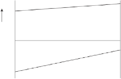
Figure 7.4
Demonstration of merit order loading
Any vertical line linking the curves will represent the cost of a given operating condition.
A sharing of the demand by the two generators is sought such that the cost is minimum. From
the diagram it is obvious that the minimum cost
C
min
occurs when the unit A takes as much
of the load share as possible, i.e. it is loaded to its maximum level, with unit B brought in to
cover the defi cit.
The
incremental cost
of a plant is provided by the slope of the cost curve, d
C
/d
P
= K
. In
the example of Figure 7.4, unit A might be a nuclear plant with very large capital costs (hence
large
K
A
) and very low fuel costs (hence low incremental cost
′
K
A
), while unit B could be a
coal fi red station with lower capital costs but higher incremental costs.
A plant loading methodology is now clear. If there are
n
plants available arrange the plants
in order of increasing K
′
, the so - called
merit order
. Starting from the top of the list, the plants
are then loaded (each up to the limit of its capacity) before the next plant on the list is brought
into action. This loading results in the scheduling shown in Figure 7.3.
To summarize, in the merit order approach, units with low operating costs run prefer-
entially and therefore attract high load factors; they generate a disproportionately large
share of electricity relative to their capacity. They are called
base load plants
, or high
merit plants. Units with high operating costs only run during peak demand, generate a
disproportionately small share of the total electricity and are known as
peaking plant
.
Plants in between these two extremes are called
intermediate plants
or middle merit
plants.
′
7.3.3 Equal Incremental Cost Dispatch
The merit order philosophy is adequate and convenient for rough scheduling but as a precise
tool of economic dispatch it is inaccurate. The reason for this is that cost curves are not quite
linear as assumed above; they are better described by a quadratic function as in the example
of Figure 7.5. Such curves can be used to determine the overall effi ciency of the plant at
various output levels.
As previously, it can be assumed that only two plants A and B are supplying a demand
P
d
. Following the plotting method in Figure 7.4, the curve for unit A is plotted in Figure 7.6
conventionally while the axis of the unit B curve is rotated by 180 °. Again the origin
O
B
of