The Optimal Set of Classifiers - Design and Analysis of Learning Classifier Systems - page 131

Prior density for classifier noise variance Prior density for classifier weight variance

0.05 0.0004

0.00035

0.04

0.0003

0.00025

0.03

0.0002

0.02

0.00015

0.0001

0.01

5e-05

0

0

0 50 100 150 200 0 5000 10000 15000 20000

Variance Variance

(a) (b)

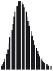
Fig. 7.3. Histogram plot of the density of the (a) noise variance, and (b) variance
of the weight vector prior. The plot in (a) was generated by sampling from τ − k and
shows that the prior on the variance is very flat, with the highest peak at a density of
around 0.04 and a variance of about 100. The plot in (b) was generated by sampling
from ( α k τ k ) − 1 and shows an even broader density for the variance of the zero mean
weight vector prior, with its peak at around 0.00028 at a variance of about 10000.

where Γ( ) is the gamma function, α k parametrises the variance of the Gaussian,

and a τ and b τ are the parameters of the Gamma distribution. This prior distribu-
tion is known as normal inverse-gamma , as the inverse variance parameter of the
Gaussian is distributed according to a Gamma distribution. Its use is advanta-
geous, as conditioning it on a Gaussian results again in a normal inverse-gamma
distribution, that is, it is a conjugate prior of the Gaussian distribution.
The prior assumes that elements of the weight vectors w jk are independent and
most likely zero, which is justified by the standardised data and the lack of further
information. Its likelihood of deviating from zero is parametrised by α k . τ k is added
to the variance term of the normal distribution for mathematical convenience, as
it simplifies the computation of the posterior and predictive density.
The noise precision is distributed according to a Gamma distribution, which
we will parametrise similar to Bishop and Svensen [20] by a τ =10 − 2 and
b τ =10 − 4 to keep the prior suciently broad and uninformative, as shown in
Fig. 7.3(a). An alternative approach would be to set the prior on τ k to express
the belief that the variance of the localised models will be most likely smaller
than the variance of a single global model of the same form. We will not follow
this approach, but more information on how to set the distribution parameters
in such a case can be found in work on Bayesian Treed Models by Chipman,
George and McCulloch [62].
We could specify a value for α k by again considering the relation between
the local models and global model, as done by Chipman, George and McCulloch
[62]. However, we rather follow the approach of Bishop and Svensen [20], and
treat α k as a random variable that is modelled in addition to W k and τ k .Itis
assigned a conjugate Gamma distribution

·

a α ,b α )= b a α α ( a α − 1)

k
Γ( a α )

p ( α k )=Gam( α k | − a α α k ) ,

exp( (7.9)