Process Observers and Data Reconciliation Using Mass and Energy Balance Equations - Advanced Control and Supervision of Mineral Processing Plants - page 71

likelihood ratio test [118] is applied to the residuals of the assumed fault subsets,
and the subset exhibiting the maximum score is assumed to be responsible for the
detected faults [70, 117].
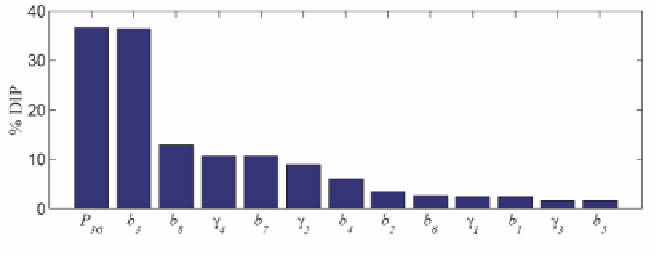
Example. Figure 2.23 gives an illustration of the method of fault isolation for the
plant of Figure 2.7. A bias that has an amplitude of three times the measurement
error standard deviation has been simulated in the sensor of stream 4 (in the data
reconciliation example of Section 2.7.2, the stream 3 metal flowrate was assumed
to be unmeasured; here all the states are measured, thus increasing the redundancy
degree). The set of potential faults consists of the biases F Y

( 1 ) to F Y ( 8 ) for the

eight streams and the node imbalances faults F X for the four nodes. The

diagnosis test is performed by sequentially splitting the fault set into one particular
fault and the remaining potential faults. Knowing the statistical properties of e and ε
as well as the fault amplitude, it is possible to calculate the probability of isolation of
the fault. This is what has been done in Figure 2.23, assuming that a 5% level of false
alarms is tolerated. It shows the probability of fault detection (D), while the other
probability bars represent the probability of diagnosing the twelve potential faults
as being the actual fault. It is clear that the assumption that the fault is in sensor
4 has the largest probability. However, wrong isolation decisions are also possible.
The isolation test performance would obviously increase if the bias were of larger
amplitude, or the data acquisition process repeated in a larger time window.

( 1 ) to F X ( 4 )

t
Figure 2.23 Probabilities of detection (D) and isolation of a bias in sensor 4, and of other potential
faults F X and F Y

Figure 2.24 shows the same bar diagram for a simulated leakage at node number
2 of Figure 2.7. The amplitude of the leakage is three times the standard deviation
of the node imbalance. Again the right diagnosis is the most probable, but wrong
fault isolations are possible.
The same method can be applied to dynamic data reconciliation [116], [119,
120]) increasing the size of the vector Y by adding past state values, or by pre-
filtering the measurements on a given past time horizon such that the node input and
output measurements are synchronized [50].