Process Observers and Data Reconciliation Using Mass and Energy Balance Equations - Advanced Control and Supervision of Mineral Processing Plants - page 38

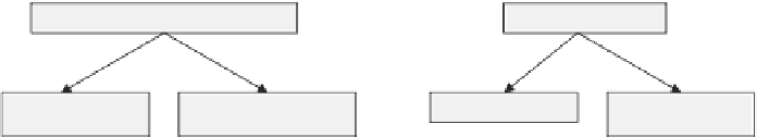
quence, others are non-observable. In fact any system of observation as depicted by
Equation 2.32 or 2.35 can be decomposed into unobservable and observable parts.
Moreover, the observable states can also be classified into minimal observability and
redundant observability classes. Figure 2.6 shows the classification tree that can be
drawn for the measured Z variables and the process states. The particular case where
measured process variables are state variables ( Z X m ) is given within brackets.

The classification of the process variables and the decomposition of the equation
system (2.32), or (2.35) in the linear case, into its redundancy part of Equation 2.37
are two related problems. The initial Equation 2.32 can be rewritten as

=

R ( Z r )= 0 ,

Q ( Q ( Q ( X o )= Z r )+ Z nr ),

(2.46)

X no ,

where the second equation corresponds to the deductible part of the system, al-
lowing calculation of the observable states X o . Various methods are available for
this decomposition of the initial system and the classification of the process vari-
ables. They have been developed mainly for linear systems, but also extended to
multi-linear systems. The graph theory is used in [65] and [66]. The Gauss Jordan
elimination technique is used in [67], projection matrices in [68] and [69], a mix-
ture of graph theory and linear algebra in [70], and the QR factorization in [71].
Using adapted process variable combinations, these methods have been extended to
bilinear systems and even to multi-linear systems [72].

Measured variables (or X m ) State variables X

Z

Redundant Not redundant Observable X o Unobservable

X no

Z r Z nr

(or X mr ) (or X mnr )

Measured
value

Measured
value

Redundant X or Not redundant X onr

Y r Y nr

Figure 2.6 Scheme showing the status of the various process variables

2.6.2 General Principles for State Estimate Calculation

The data reconciliation problem to be solved is schematically represented in Figure
2.5, where the known information is given at the reconciliation procedure input
and the process states to be estimated at the procedure output. When f and g are
linear functions and inequality constraints are inactive, the solution to this problem
is analytical. This occurs when the measured process variables are plant states or