Environmental Engineering Reference
In-Depth Information
empirical models have been used for simulating crushing plants, with excellent re-
sults for operational purposes [7, 8]. On the other hand, there have been few studies
on models based on first principles;
i.e.
, mechanical laws [9]. These models, which
are usually more complex, describe in detail the factors affecting the reduction pro-
cess. Their use is oriented to the design and optimization of crusher structure. Semi-
empirical models provide a reasonable compromise between representability and
simplicity. For this reason, the model used in the simulator is based on Whiten's
perfect mixing model [7].
feed
Flowrate
f
Size distribution
f
Hardness γ
f
product
Flowrate
p
Size distribution
p
Hardness
γ
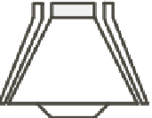
Figure 5.2
A cone crusher and its main variables
The variables associated to the crusher model are depicted in Figure 5.2. Mass
balance of the contents is given by the following equation [7]:
d
m
(
t
)
=
f
(
t
)−
p
(
t
)−
γ
(
t
)(
S
−
BS
)
m
(
t
),
(5.1)
dt
where γ
(
t
)
is a variable representing ore hardness,
f
(
t
)
and
p
(
t
)
are vectors having
as elements
f
i
, which are the mass flowrate in the
i
th size fraction of the
feed and the product, respectively. The mass in the
i
th size fraction of the contents is
noted as
m
. The matrix
S
is a diagonal matrix representing the specific breakage rate
of size
i
,
B
is a lower diagonal matrix, where
b
ij
represents the fraction of particles
of size fraction
j
appearing in the size fraction
i
after breakage. Product mass flow
is assumed to be proportional to the mass contents;
i.e.
,
(
t
)
and
p
i
(
t
)
p
=
Dm
,
(5.2)
where
D
is a diagonal matrix representing each element in the specific discharge rate
of size
j
. The steady-state solution of (5.1) can be found by setting the first term to
zero and expressing
p
in terms of
f
as follows:
]
−
1
f
p
=[
I
−
C
][
I
−
CB
,
(5.3)


Search WWH ::

Custom Search