Introduction to Power Pivot - Microsoft Business Intelligence Tools for Excel Analysts - page 45

If the Power Pivot tab does not appear on the Ribbon, close and restart Excel 2013.
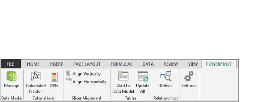
After installing the add-in, the Power Pivot tab appears on the Ribbon, as shown in Figure 3-1.
Figure 3-1: After you activate the add-in, you see the Power Pivot tab on the Ribbon.
The Power Pivot Ribbon interface exposes the full set of functionality you don't get with the standard
Data tab. Here are a few examples of functionality available with the Power Pivot interface:
➤ Browse, edit, filter, and custom sort data import.
➤ Create custom calculated columns that apply to all rows in your data import.
➤ Define a default number format to use when the field appears in a PivotTable.
➤ Configure relationships via a handy graphical diagram view.
➤ Prevent certain fields from appearing in the PivotTable Field List.
➤ Configure specific fields to be read as Geography or Image fields.
➤ Access Key Performance Indicators (KPI).
Linking Excel Tables to Power Pivot
The first step in using Power Pivot is to fill it with data. You can either import data from external data
sources or link to Excel tables in your current workbook. See Chapter 4 for more about importing
data from external data sources. For now, you can link three Excel tables to Power Pivot.
In this scenario, you have three datasets in three different worksheets (see Figure 3-2):
➤ The Customers dataset contains basic information like CustomerID, CustomerName, and Address.
➤ The InvoiceHeader dataset contains data that points specific invoices to specific customers.
➤ The InvoiceDetails dataset contains the specifics of each invoice.
If you want to analyze revenue by customer and month, you need to join these three tables. In the
past, you'd have to go through a series of gyrations involving vlookup or other clever formulas. But
with Power Pivot, you can build these relationships in just a few clicks.