PivotTable Fundamentals - Microsoft Business Intelligence Tools for Excel Analysts - page 34

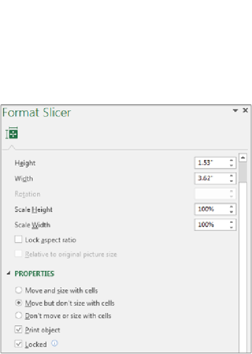
You can then adjust the size of the slicer in the Format Slicer pane shown in Figure 2-24. You can
specify how the slicer should behave when cells are shifted and specify whether the slicer should be
shown when printed.
Figure 2-24: Use the Slicer Format pane to adjust how the slicer behaves in relation to the worksheet it's on.
Data item columns
By default, all slicers are created with one column of data items. You can change this by right-clicking
the slicer and selecting Size and Properties. In the Position and Layout section of the Format Slicer pane,
you can specify the number of columns in the slicer. Adjust the number to 2 (as shown in Figure 2-25)
and the data is displayed in two columns, adjust the number to 3 and the data is displayed in three
columns, and so on.
Slicer color and style
To change the color and style of your slicer, click it, and then select a style from the Slicer Style gallery
on the Slicer Tools Options tab. The default styles available suit a majority of dashboards, but if you
want more control over the color and style of your slicer, you can click the New Slicer Style button on
the lower left-hand corner. You can then specify the detailed formatting of each part of the slicer.
Other slicer settings
Right-click your slicer and select Slicer Settings to open the Slicer Settings dialog box. With this dialog
box, you can control the look of your slicer's header, how your slicer is sorted, and how filtered items
are handled.
With minimal effort, your slicers can be integrated nicely into your dashboard layout. Figure 2-26
shows how two slicers and a chart work together as a cohesive dashboard component.