Information Technology Reference
In-Depth Information
Table 3.35.
EDE comparison with
DE
spv
and PSO over the Taillard benchmark problem
GA
PSO
spv
DE
spv
DE
spv
+
exchange
EDE
Δ
avg
Δ
std
Δ
avg
Δ
std
Δ
avg
Δ
std
Δ
avg
Δ
std
Δ
avg
Δ
std
20x5
3.13
1.86
1.71
1.25
2.25
1.37
0.69
0.64
0.98
0.66
20x10
5.42
1.72
3.28
1.19
3.71
1.24
2.01
0.93
1.81
0.77
20x20
4.22
1.31
2.84
1.15
3.03
0.98
1.85
0.87
1.75
0.57
50x5
1.69
0.79
1.15
0.7
0.88
0.52
0.41
0.37
0.4
0.36
50x10
5.61
1.41
4.83
1.16
4.12
1.1
2.41
0.9
3.18
0.94
50x20
6.95
1.09
6.68
1.35
5.56
1.22
3.59
0.78
4.05
0.65
100x5
0.81
0.39
0.59
0.34
0.44
0.29
0.21
0.21
0.41
0.29
100x10 3.12
0.95
3.26
1.04
2.28
0.75
1.41
0.57
1.46
0.36
100x20 6.32
0.89
7.19
0.99
6.78
1.12
3.11
0.55
3.61
0.36
200x10 2.08
0.45
2.47
0.71
1.88
0.69
1.06
0.35
0.95
0.18
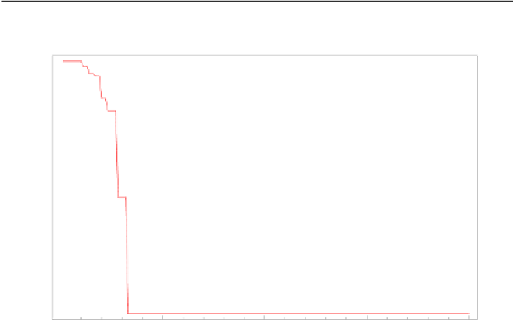
F 30 x 100 History
920
900
880
860
840
820
0
50
100
150
200
Number of Generations
Fig. 3.15.
Sample output of the F30x100 FSS problem.
The third experimentation module is referenced from [37]. These sets of problems
have been extensively evaluated (see [22, 34]). This benchmark set contains 100 par-
ticularly hard instances of 10 different sizes, selected from a large number of randomly
generated problems.
A maximum of ten iterations was done for each problem instance. The population
was kept at 100, and 100 generations were specified. The results represented in Table
3.35, are as quality solutions with the percentage relative increase in makespan with
respect to the upper bound provided by [37] as given by Equation 3.10.


Search WWH ::

Custom Search