Discrete Set Handling - Differential Evolution: A Topic for Global Permutation-Based Combinatorial Optimization - page 182

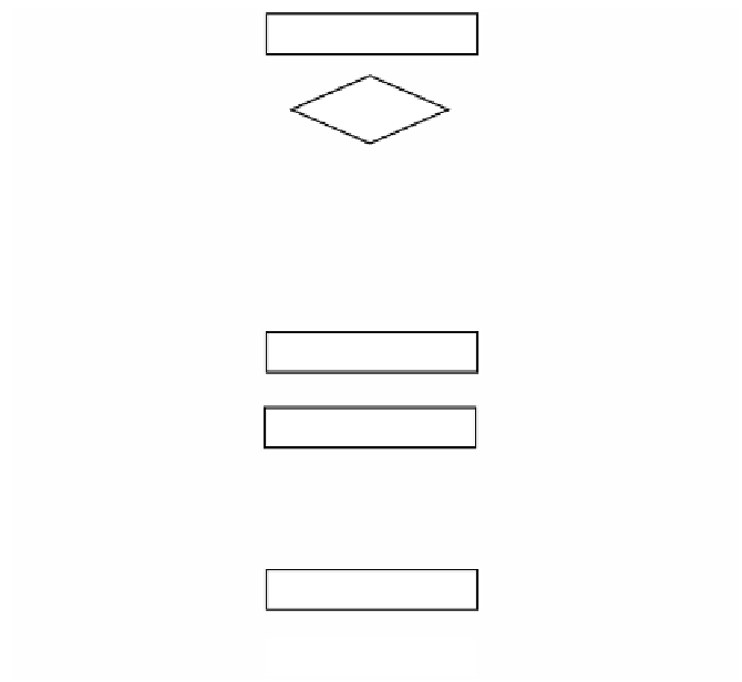
Fig. 7.34. Data flow diagram of DE

CostFunction Compile Solution, Integer, 1 , Prob, Integer, 2 , Mach, Integer ,
Module JTime, LMach ,
JTime Accumulate & Prob 1, & Solution ;
LMach Accumulate & Prob , Solution 1 & Range Mach ;
Table JTime 1 LMach i 1 ;
MapIndexed JTime First 2 1 Max JTime First 2 , JTime First 2 1
Prob i 1, 1 &, Rest Solution , i, Mach 1 ; Return JTime 1

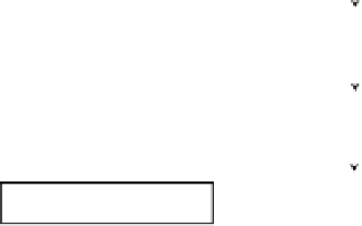
Fig. 7.35. Flow Shop Schedluing routine

Max[JTime[[First[#2]]] , JTime[[First[#2]+1]]] + Prob[[i + 1 , #1]])& , Rest[Solution]],the
processing time value is simply accumulated in LMach .
For more information about Flow Shop, please see [17].

7.4.2 DE Traveling Salesman Problem

The Traveling salesman function is simply the accumulation of the distances from one
city to the next. The function is given in Fig 7.36.
The first routine simply picks up the times between the cities in the Solution .The
distance times are stored in the matrix Distance .
Time+=(Distance[[Solution[[# + 1]] , Solution[[#]]]])& / @Range[Size

− 1];.