Geology Reference
In-Depth Information
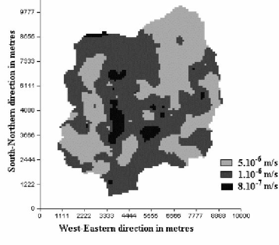
Figure 5.
Hydraulic conductivities in the weathered
layer, after calibration.
Figure 5 shows the distribution of the calibrated hydraulic conductivities
for the weathered layer. They range between 8.10
-7
m.s
-1
and 5.10
-6
m.s
-1
.
The transmissivities were calculated from the results of 34 aquifer tests in
the weathered-fissured granite layer. But the high variability observed in the
field and the difficulties of matching the simulated heads with the measured
ones led to additional manual calibration of the hydraulic conductivities in
the model.
Average hydraulic conductivity obtained by calibration was compared
with the equivalent horizontal hydraulic conductivity calculated by the
FRACAS model (Bruel et al., 2002), a “discrete fracture network” model,
which was used to interpret 25 slug tests. The hydraulic conductivities in the
weathered-fissured granite layer are shown in Figure 6. They exhibit large
variability (1.10
-7
to 3.10
-5
m.s
-1
) from one place to another because of the
heterogeneity of the rocks.
In the weathered-fissured granite layer, linear heterogeneities (impervious
vertical barriers) had to be introduced into the model because this was the
only way to take into account the observed piezometric data. These
heterogeneities were attributed to the dykes that crop out in the studied area,
to a South-North quartz reef crossing the watershed and to some assumed
extensions of dykes (Fig. 6).
The specific yield was taken to be 2.4% in the weathered rocks. This
value is an average of the specific yields observed in the weathered rocks