Analysis of Uncertain Scalar Data with Hixels - Scientific Visualization: Uncertainty, Multifield, Biomedical, and Scalable Visualization - page 35

76

0

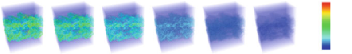
Fig. 3.2 Varying areal persistence and its effect on bucketing for the Jet dataset. Using hixels
with size 16 3 and 256 bins/histogram, we vary areal persistence for all powers of two between 16
and 512, inclusive, from left to right . Color indicates how many buckets at that hixel's position in
( x , y , z ) space. At low levels of persistence, as many as 76 buckets can be selected in the hixel, but

as persistence increases, most hixels have only 1 or 2 buckets. ©IEEE reprinted, with permission,
from Thompson et al. [ 10 ]

3.2 Analysis of Hixel Data

In this section we summarize algorithms (1) to extract approximations of common
topological structures from hixel data; (2) to segment multi-modal data by splitting
individual histograms into their modes and correlate neighboring modes; and (3) to
define and render uncertain isosurfaces.

3.2.1 Sampled Topology

Hixels encode potential scalar values along with their distributions at sample loca-
tions, and thus can aid visualization of the uncertainty in topological segmentations
of down-sampled data. We use a three step process where we (1) sample the hixels
to generate individual instances of the coarser representation, (2) compute the Morse
complex on the instance, and (3) aggregate multiple instances of the segmentation
to visualize its variability. We generate an instance V i of the down-sampled data by
picking values at each sample location from the co-located hixel. The value is picked
at random, governed by the distribution encoded by the hixel. By picking values in-
dependently from neighboring values, we can simulate any possible down-sampling
of the data, assuming each hixel's distribution is independent.
For each sampled field V i we compute the Morse complex of the instance using
a discrete Morse theory based algorithm [ 5 ], and identify basins around minima for
varying persistence simplification thresholds. We next create a binary field C i that
encodes the geometric information of the arcs of the complex. Each sample location
in V i contributes a value of 1 to C i if the sample is on the boundary of two or more
basins, otherwise it contributes 0 if the sample is in the interior of a basin.
To visualize the variability of the topological segmentation of sub-sampled data,
we repeatedly sample the hixels producing V i 's, and compute their basin boundary
representations C i .After n iterations, an aggregate function is computed over the
boundary representations, recording the fractional identification of a sample location