Image Processing Reference
In-Depth Information
(a)
(b)
upper outliers (%)
0%
25%
25%
0%
lower outliers (%)
10
20
l
a
t
i
t
u
d
e
Pacific
total outliers (%)
Indian
Atlantic
-20
-10
0
10
20
median temp.
(c)
(d)
1
measure of outlyingness
3.5
2.0
0.5
2.54
-2.54
12
2
4
6
8
10
14
1
18
20
22 24
26
28
30
distance to median temp.
-0.5
total outliers (%)
-2.0
-3.5
-1
(f)
(e)
Pa
cif
ic
I
nd
ia
n
A
tla
nti
c
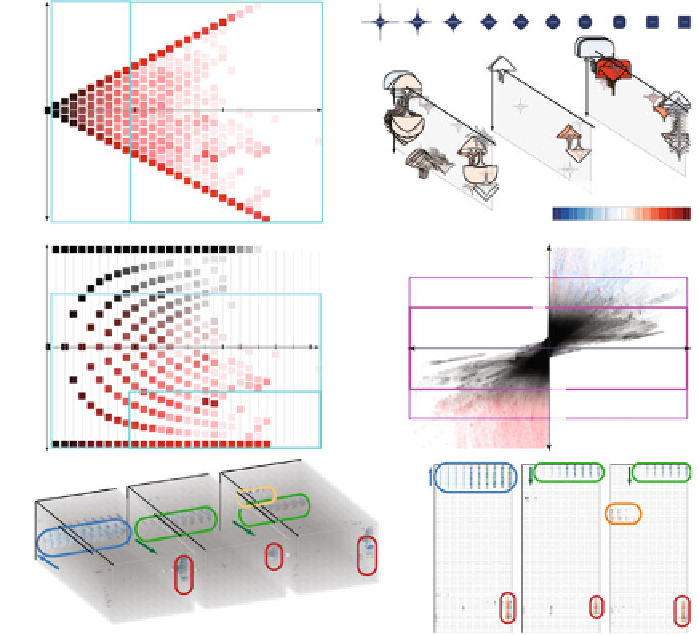
Fig. 15.4
Selected steps within a complex analysis example (outlier analysis in a multi-run climate
simulation dataset—more details in the main text). After having used the interactive data derivation
mechanism to compute an IQR-based outlyingness measure, spatiotemporal locations are identified
with outliers. This identification is achieved by brushing scatter plot (
a
) and observing the selected
locations in the linked visualization (
b
). In a next step, the analysis was confined to lower-value
outliers (using the data derivation mechanism, again) by brushing scatterplot (
c
). Subsequently, to
see the actual outliers themselves, a new scatter plot was used, with detrended and accordingly
normalized temperature values on
y
, to focus on the actual outliers, then observed in views (
e
)and
(
f
). More details about this study are available in the main text and in a paper by Kehrer et al. [
16
]
Up to this point, the entire analysis was solely focused on delimiting locations that
have outliers of a particular characteristic. In the next step, the focus was directed to
the outliers themselves. To select them, another data derivation steps was performed,
computing detrended and normalized temperature values per location (the performed
operation was to first subtract the median temperature wrt. all simulation runs, per
location, and then divide by IQR). A new scatter plot, shown in Fig.
15.4
(d), was used
to show all data points wrt. their distance to the median (
x
-axis) and this detrended and
normalized temperature measure (
y
-axis). Consistent with Fig.
15.4
a, b, all points
Search WWH ::

Custom Search