Derived Fields - Scientific Visualization: Uncertainty, Multifield, Biomedical, and Scalable Visualization - page 142

(a) (b) (c) (d)

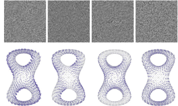
Fig. 14.8 Two examples of Hodge-Helmholtz decomposition: ( top ) a planar vector field, and ( bot-
tom ) a vector field defined on a torus. From left to right are: ( a ) the original field V ,( b ) the curl-free
component V c ,( c ) the divergence-free component V d , and the harmonic component V h . Notice that
singularities in the original field can be captured effectively by the decomposition. Moreover, the
harmonic component is more prominent for fields defined on a hyperbolic manifold. Image courtesy
of Polthier and Preuss [ 18 , 19 ]

smooth vector field on a genus-two surface must contain at least four saddles or some
higher-order saddles.
Polthier andPreuss develop techniques to efficiently performtheHodge-Helmholtz
decomposition on a triangular mesh with a piecewise constant vector field [ 18 , 19 ]
(Fig. 14.8 ). Such techniques are later extended to volumes [ 25 ].
Another important application of the Hodge-Helmholtz decomposition is in fluid
simulation. In this case the fluids are assumed to divergence-free. However, numerical
solvers often introduce errors which lead to flow fields with a non-zero divergence,
thus causing unrealistic fluid behaviors. This is corrected by a projection step, for
which the Hodge-Helmholtz decomposition is performed on the vector field, and the
curl-free part is removed [ 23 , 24 ].

14.4.2 Components of Tensor Field

There has been some recent trend in studying asymmetric tensor fields [ 1 , 13 , 28 ,
29 ], with applications in flow visualization and earthquake engineering. Given a
vector field V such as the velocity of fluid particles or the deformation of land, the
gradient T V is an asymmetric tensor field which can be used to describe the

deformation of particles in both fluid and solid movements. This can be explained

=