Biology Reference
In-Depth Information
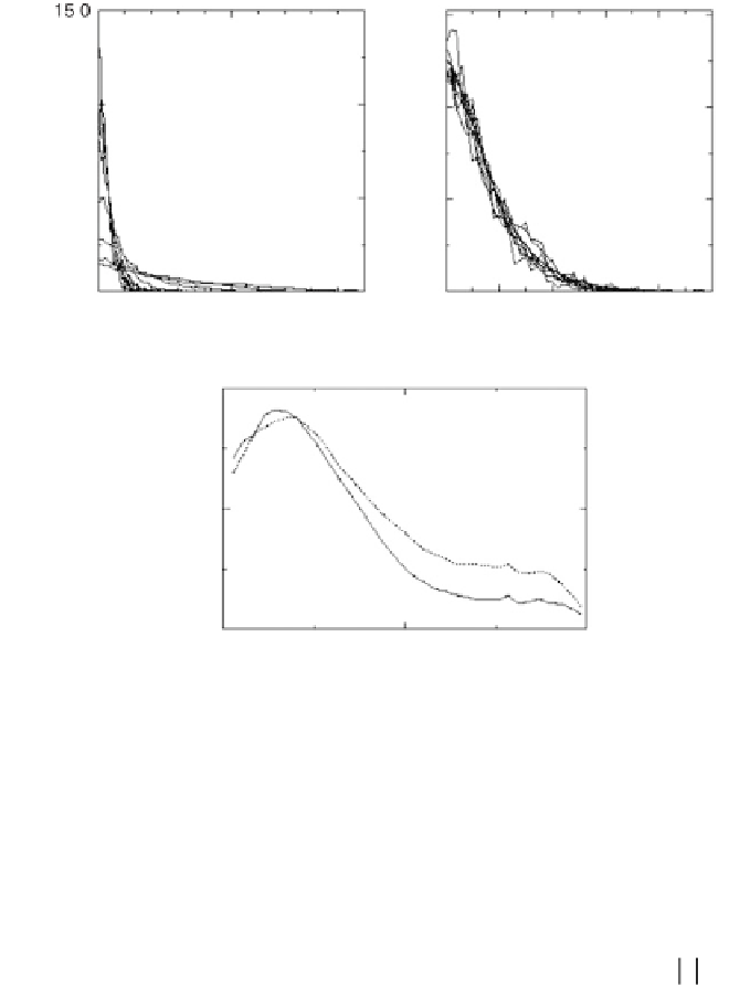
Figure 4.3
The noise distribution functions at different values of mean
expression values: q
0
=
0.9, 1.3, 1.7, 2.2, 2.6, 3, 3.5, 3.9 (a) before and (b) after
rescaling by the standard deviation s
2
(
, which is shown in (c). Only the
positive region of is shown in (a) and (b) for symmetry reasons. The
rescaled distribution functions collapse onto a single curve well fitted by
plotted as the thick line shown in (b).
q
0
)
δθ >
0
2
Φ
()
x
=
05
. exp(
−
x
/.
05
+
06
.
x
)
contrast with a Gaussian distribution. In fact,
Φ
(x)
can be approximated
very well by an empirical function
Φ
()
x
≈
05
. exp(
−
x
2
05 06
.
+
.
x
)
as
shown in figure 4.3b (thick solid line).
From eq. (2), one observes that all of the expression-dependent
information in the noise is given by the variance for . The
following subsection focuses on analyzing the dependence of the noise
strength
2
σ
()
θ
θ
0
≥
1
0
2
σ
()
θ
on the expression value.
0
NOISE DUE TO SAMPLE PREPARATION AND HYBRIDIZATION
To dissect the origins of noise, the total measurement noise is divided into
two parts: the first is sample preparation noise dq
prep
caused by the prehy-
bridization steps such as reverse transcription and IVT; the second is the


Search WWH ::

Custom Search