Biomedical Engineering Reference
In-Depth Information
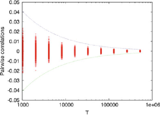
Fig. 8.6
Correlation (
8.12
) as a function of sample length
T
in a model where spikes are
independent. For each
T
we have generated
1
,
000
rasters of length
T
, with two independent
neurons, drawn with a firing rate
p
=
1
2
. For each raster we have computed the pairwise
correlation (
8.12
) and plotted it in log-scale for the abscissa (
red point
). In this way we have a
view of the fluctuations of the empirical p
airwise co
rrelation about it
s (zero) ex
pectation. The full
lines represent respectively the curves
3
p
2
(1
−p
2
)
T
p
2
(1
−p
2
)
T
(
green
) accounting
for the Gaussian fluctuations of
C
(
T
ω
(
k,j
)
:
99 %
of the
C
(
T
ω
(
k,j
)
's values lie between these
two curves (called “confidence bounds”)
(
blue
)and
−
3
independent, the quantity
C
(
T
)
(
k,j
) will in general not be 0:ithas
fluctuations
ω
around 0.
This can be seen by a short computer program drawing at random 0's and 1's
independently, with the probability
p
tohavea'1', and plotting
C
(
T
)
(
k,j
) for
ω
different values of
ω
, while increasing
T
(Fig.
8.6
).
As a consequence, it is stricto-sensu not possible to determine whether random
variables are uncorrelated, by only computing the empirical correlation from
samples of size
T
, since even if these variables are uncorrelated, the empirical
correlation will never be zero. There exist statistical tests of independence from
empirical data, beyond the scope of this chapter. A simple test consists of
p
lotting
the empirical correlation versus
T
and check whether it tends to zero as
T
.Now,
experiments affords only s
am
ple of limited size, where
T
rarely exceeds 10
6
.So,
fluctuations are of order
√
K
×
10
−
3
and it makes a difference whether
K
is small
or large.
It is therefore difficult to interpret
weak
empirical correlations. Are they sample
fluctuations of a system where neurons are indeed independent, or are they really
significant, although weak? This issue is further addressed in Sect.
8.4.2
.

Search WWH ::

Custom Search