Biomedical Engineering Reference
In-Depth Information
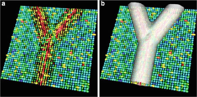
Fig. 6.9
Tensor field segmentation on a synthetic dataset simulating DTI [
41
]. (
a
) A slice from
a
40
×
40
×
40
dataset of synthetic diffusion tensors composed by a
divergent
tensor field and
a background of isotropic tensors. Within the
Y
shape FA decreases as one gets further from the
center-line. Noise was added to the original dataset. The colour of the tensors represent anisotropy
with
red
indicating high anisotropy and
blue
indicating isotropy. (
b
) The segmented divergent
Y
shape using the level-set approach
segmentation boundary. Therefore, a DT at the point
x
in the image corresponds
to the 3D Gaussian distribution
N
(
x, r
)
.
Using the level-set approach and the optimal boundary
Γ
between the object of
interest
Ω
1
and the background
Ω
2
, the level-set
φ
:
Ω
1
∪ Ω
2
→
R
can be defined as:
⎧
⎨
φ
(
x
)=0
,
if
x
∈
Γ
(6.30)
φ
(
x
)=
D
E
(
x, Γ
)
,
if
x
∈
Ω
1
⎩
φ
x
)=
−D
E
(
x, Γ
,
x
∈
Ω
2
(
)
if
where
represents the Euclidean distance between
x
and
Γ
. Then accord-
ing to the geodesic active regions model along with a regularity constraint on the
interface, the optimal boundary
Γ
or the segmentation of the tensor field is obtained
by minimizing the functional:
E
(
φ, P
1
,P
2
)=
ν
D
E
(
x, Γ
)
Ω
=
Ω
1
∪Ω
2
|∇H
ε
(
φ
)
|dx −
H
ε
(
φ
)ln(
P
1
(
N
(
x, r
)))
dx
Ω
Ω
(1
−
−
H
ε
(
φ
)) ln(
P
2
(
N
(
x, r
)))
dx,
(6.31)
where
H
ε
(
·
)
is a regularized version of the Heaviside function [
23
], and
P
1
and
P
2
are the probability distributions of the set of Gaussian distributions
N
x, r
in
Ω
1
(
)
and
Ω
2
respectively.
Equation (
6.31
) can be solved computationally by assuming the distributions
P
1
and
P
2
themselves to be Gaussians distributions. However, that would require
Search WWH ::

Custom Search