Deconvolution and Denoising for Confocal Microscopy - Modeling in Computational Biology and Biomedicine - page 141

Algorithm 7 The RL-TV deconvolution algorithm
Input: Observation i ( x ) ∀ x ∈ Ω s , background b ( x ) ≥ 0, regularization parameter λ ∈ R

+ ,

+ .
Output: Restored specimen o ( x ).
1: Calculate PSF h ( x ) ∈O (Eq. 4.5 ),
2: Initialize: n ← 0, o

criterion ε ∈ R

( n ) ( x ) ← Mean( i ( x )).

( n ) ( n− 1) ( n )

3: while |o ≥ ε do − o |/o

{ Calculate div( ∇o n ( x ) /|∇o n ( x ) | ε ) by the minmod scheme. }

4:

( n +1) ( x ) by Eq. ( 4.29 ). }

5:

{ Deconvolve: o

( n +1) ( x ) for

6:

{ Sub-space

projection (scale): o total number of photons preservation

x o

( n ) ( x )=

x i ( x ) }

( n +1) ( x ) < 0 to zero. }

7:

{ Sub-space projection (positivity): Set o

( n ) ( x ) ← o ( n +1) ( x ) and n ← ( n +1) . }

8:

{ Set: o

9: end while

400

Original bead
Blurred bead
Observed bead
Restored bead

350

300

250

200

150

100

50

0

1 20 39 58 77 96 115

X

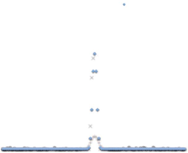
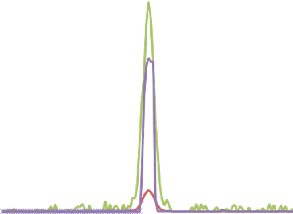
Fig. 4.10 Comparison of the radial intensity profiles for an original 100 nm fluorescent sim-
ulated bead sample, the blurred bead without any noise, the observed bead (after removing
the background), and the restored bead using deconvolution. The result was obtained with a
regularization parameter λ =0 . 002, and the iterations were terminated at the 100th iteration while
the convergence was after about 50 iterations

In addition to simulated data, we tested the algorithm on the Convallaria
specimen of Fig. 4.3 b in Sect. 4.2.1.1 . This thin sample was imaged using a