Agriculture Reference
In-Depth Information
0
0.2
0.4
0.6
0.8
1
0
0.2
0.4
0.6
0.8
1
x
x
0
0.2
0.4
0.6
0.8
1
0
0.2
0.4
0.6
0.8
1
x
x
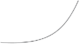
Figure 10.6
Different types of curves. The top two are examples of power curves. The lower left
is a decay curve and the lower right is a growth curve.
The ANOVA command allows there to be both continuous and
categorical predictors in the same analysis. The
c.
before a variable
tells the program to treat this variable as continuous, as it would be
treated in a simple regression analysis. In addition, the
days
vari-
able is entered as a categorical variable. This analysis suggests that
the regression has continuous variable
days
not significant (P>F =
0.1091) while the categorical
days
variable is significant indicating
the regression is not linear. The R
2
in this case is greater than the
previous analysis suggesting this is a better fit.
Clearly ambiguous results such as this suggest more work should be
done. Perhaps a single onion variety could be harvested over an extended
period of time and analyzed for pungency to get a clearer understanding.
Not all relationships are linear, but may follow some other func-
tional relationship. Figure 10.6 shows several graphs of functions that
may be encountered in agricultural studies. Datasets that appear to
follow one of these graphs may be analyzed with linear regression
after the data have been transformed using a log transformation.
Open the dataset Onion Bulb Sizes.dta. This is a dataset from Little
and Hills (1978, p. 199). Graphing this datum indicates an increase in


Search WWH ::

Custom Search