Information Technology Reference
In-Depth Information
Given an error bound
ε
, we can choose a suciently small step duration
δ>
0
such that
p
P
max
s,
(
k
a
,k
b
]
−
p
max
(
s, I
)
≤
(
λδ
)
2
2
+
λδ < ε
holds. Note that
k
b
·
this can be done
apriori
. Hence,
p
P
max
s,
(
k
a
,k
b
]
approximates the probabilities
p
max
(
s, I
)upto
ε
.Further,
p
P
max
s,
(
k
a
,k
b
]
can easily be computed by slightly
adapting the well-known value iteration algorithm for MDPs [7]. For an error-
bound
ε>
0andatime-interval
I
with sup
I
=
b
, this approach has a worst
case time complexity in
(
λb
)
2
/ε
where
λ
is the maximal
exit rate and
m
and
n
are the number of transitions and states of the IMC,
respectively.
n
2
.
376
+(
m
+
n
2
)
O
·
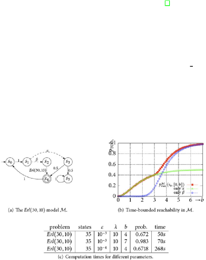
Example 3.
(Adopted from [58].) Consider the IMC depicted in Fig. 2(a). Let
G
=
as indicated by the double-circled state
s
4
. The only state which
exhibits non-determinism is state
s
1
where a choice between
α
and
β
has to be
made. Selecting
α
rapidly leads to the goal state as with probability
2
,
s
4
is
reached with an exponential distribution of rate one. Selecting
β
almost surely
leads to the goal state, but, however, is subject to a delay that is governed by
an Erlang(30,10)-distribution, i.e., a sequence of 30 exponential distributions of
each rate 10. Note that this approximates a deterministic delay of 3 time units.
The time-bounded reachability probabilities are plotted in Fig 2(b). This plot
clearly shows that it is optimal to select
α
upto about time 3, and
β
afterwards.
The size of the IMC, its maximal exit rate (
λ
), accuracy (
), time bound (
b
)and
the computation time are indicated in Fig. 2(c).
{
s
4
}
Fig. 2.
Time-bounded reachability probabilities in an example IMC
Time-bounded reachability-avoid probabilities.
To conclude this section, we will
explain that determining
p
max
(
s, I
) can also be used for more advanced measures-
of-interest, such as “reach-avoid” probabilities. Let, as before,
s
be a state in an